Download
1 / 5
50 likes | 61 Views
Coherent Structures in Convective Boundary Layers. by Ernest Agee, Suzanne Zurn-Birkhimer and Alex Gluhovsky.

E N D
Coherent Structures in Convective Boundary Layers by Ernest Agee, Suzanne Zurn-Birkhimer and Alex Gluhovsky
Although there is no definitive definition of Coherent Structures (CSs), the authors elect to define CSs as structures in atmospheric flows with spatial organization. For moderately large Reynolds numbers one can possibly view flows as temporally chaotic, but spatially organized. It can also be argued that CSs may (or may not) be part of turbulence. Wintertime cold air outbreaks (CAOs) of polar continental air over extensive bodies of warmer water can create interesting spatially organized cloud patterns within convective boundary layers (see Agee, et al. 2000). Such examples of 2-d and 3-d co-existing patterns of mesoscale cellular convection can be seen in Figure 1, which are offered as examples of CSs. Yet smaller scales of CSs can be seen in similar CAO events, as shown in Figure 2 (see Mayor and Eloranta, 2001), during westerly flow off the Wisconsin shoreline over Lake Michigan. Microscale examples of coherent structures (CS1 and CS2) are identified in Figure 2, which emerge within the pattern of lake surface steam fog (again as co-existing 2-d and 3-d patterns). Field programs such as Lake-ICE (see Kristovich, et al. 2000) are providing useful special field data sets to study these spatially organized patterns. Large Eddy Simulation (LES) has also been employed by the Purdue Group (Zurn-Birkhimer, et al. 2004) to study the delicate balances that can exist between the forcing by buoyancy 'versus' shear in the evolution of 2-d and 3-d patterns of CSs at different length scales, times scales, and spatial distributions within the CBL. Figure 3 shows a LES-derived CBL with a pattern of CSs for moderate surface heat flux and moderate wind shear. It is noted that at heights of 22m above lake level, microscale 3-d structures are evident, however at 100m ASL the pattern is a much larger co-existing structure of 3-d convection. The Purdue Group is supported in part by NSF, and is committed to understanding the evolution of coherent structures in convective planetary boundary layers, from the smallest scale beyond noise (and turbulence) to successive larger spatial scales and their predictability
Figure 1. Cold air (A or cP) advecting southeastward from the frozen Baffin Bay region to the south of Greenland and over the open waters of the North Atlantic. Notice 2-d banding giving way downstream to 3-d convective cells and chains. (NOAA-7 visible satellite image at 1606/1422 GMT on 10 March 1982 taken from Scorer, 1986).
Figure 2. CS1 embedded within CS2 identified in visual photography. An example of CS2 is outlined with the dotted line in the top image. The inset photograph was enhanced to show CS1 in detail (photograph by Dave Rogers, CSU, taken at 575m ALS, near the Wisconsin shoreline). CS2 CS1
Figure 3. Model Run 5 vertical velocity fields for surface heat flux of 400 K m s-1 and winds at x = 5 m s-1 and y = -5 m s-1. Top plots are plan views of vertical velocity with blue upward motion and red downward motion at 22 m and 100 m, respectively. The bottom graph is a plan view (from above, looking down) for the w = 1 m s-1 contour.