Download
1 / 27
310 likes | 795 Views
Atmospheric boundary layers and turbulence I. Wind loading and structural response Lecture 6 Dr. J.D. Holmes. Atmospheric boundary layers and turbulence. Wind speeds from 3 different levels recorded from a synoptic gale. Atmospheric boundary layers and turbulence.

E N D
Atmospheric boundary layers and turbulence I Wind loading and structural response Lecture 6 Dr. J.D. Holmes
Atmospheric boundary layers and turbulence Wind speeds from 3 different levels recorded from a synoptic gale
Atmospheric boundary layers and turbulence Features of the wind speed variation : • Increase in mean (average) speed with height • Turbulence (gustiness) at each height level • Broad range of frequencies in the fluctuations • Similarity in gust patterns at lower frequencies
Atmospheric boundary layers and turbulence • Mean wind speed profiles : • Logarithmic law 0 - surface shear stressa - air density u = friction velocity = (0/a) integrating w.r.t. z :
Atmospheric boundary layers and turbulence • Logarithmic law • k = von Karman’s constant (constant for all surfaces) • zo = roughness length (constant for a given ground surface) logarithmic law - only valid for z >zo and z < about 100 m
Atmospheric boundary layers and turbulence • Modified logarithmic law for very rough surfaces (forests, urban) • zh= zero-plane displacement zh is about 0.75 times the average height of the roughness
Atmospheric boundary layers and turbulence • logarithmic law applied to two different heights • or with zero-plane displacement :
Atmospheric boundary layers and turbulence • Surface drag coefficient : Non-dimensional surface shear stress : from logarithmic law :
Atmospheric boundary layers and turbulence • Terrain types :
Atmospheric boundary layers and turbulence • Power law • = changes with terrain roughness and height range zref = reference height
Atmospheric boundary layers and turbulence • Matching of power and logarithmic laws : zo = 0.02 m = 0.128 zref = 50 metres
Atmospheric boundary layers and turbulence • Mean wind speed profiles over the ocean: • Surface drag coefficient () and roughness length (zo) vary with mean wind speed (Charnock, 1955) g- gravitational constanta- empirical constant a lies between 0.01 and 0.02 substituting : Implicit relationship between zo and U10
Atmospheric boundary layers and turbulence • Mean wind speed profiles over the ocean: Assumeg = 9.81 m/s2 ;a= 0.0144 (Garratt) ; k =0.41 Applicable to non-hurricane conditions
Atmospheric boundary layers and turbulence • Geostrophic drag coefficient • Relationship between upper level and surface winds : Rossby Number : balloon measurements : Cg = 0.16 Ro-0.09 (Lettau, 1959) Can be used to determine wind speed near ground level over different terrains : Log law Lettau Lettau Log law U10, terrain 1 u*,terrain 1 Ug u*,terrain 2 U10, terrain 2
Atmospheric boundary layers and turbulence • Aircraft flights down to 200 metres • Mean wind profiles in hurricanes : • Drop-sonde (probe dropped from aircraft - tracked by satellite) : recently started • Sonic radar (SODAR) measurements in Okinawa • Tower measurements • not enough • usually in outer radius of hurricane and/or higher latitudes
North West Cape US Navy antennas Exmouth EXMOUTH GULF 100 km Atmospheric boundary layers and turbulence • Mean wind profiles in hurricanes : • Northern coastline of Western Australia • Profiles from 390 m mast in late nineteen-seventies
Atmospheric boundary layers and turbulence • Mean wind profiles in hurricanes : • In region of maximum winds : steep logarithmic profile to 60-200 m • Nearly constant mean wind speed at greater heights for z < 100 m Uz =U100 forz 100 m
Atmospheric boundary layers and turbulence • Doppler radar • Mean wind profiles in thunderstorms (downbursts) : • Some tower measurements (not enough) • Horizontal wind profile shows peak at 50-100 m • Model of Oseguera and Bowles (stationary downburst): r - radial coordinate R - characteristic radius z* - characteristic height out of the boundary layer - characteristic height in the boundary layer - scaling factor
Atmospheric boundary layers and turbulence Model of Oseguera and Bowles (stationary downburst) : • Mean wind profiles in thunderstorms (downbursts) : R = 1000 m r/R = 1.121 z* = 200 metres = 30 metres = 0.25 (1/sec)
Atmospheric boundary layers and turbulence Add component constant with height (moving downburst) : • Mean wind profiles in thunderstorms (downbursts) : R = 1000 m r/R = 1.121 z* = 60 metres = 50 metres = 1.3 (1/sec) Uconst = 35 m/s
Atmospheric boundary layers and turbulence Turbulence represents the fluctuations (gusts) in the wind speed It can usually be represented as a stationary random process
u(t) - longitudinal - parallel to mean wind direction • - parallel to ground (usually horizontal) • v(t) - parallel to ground - right angles to u(t) • w(t) - right angles to ground (usually vertical) w(t) v(t) U+u(t) ground Atmospheric boundary layers and turbulence Components of turbulence :
Atmospheric boundary layers and turbulence Turbulence intensities : • standard deviation of u(t) : Iu = u /U (longitudinal turbulence intensity)(non dimensional) Iv = v /U (lateral turbulence intensity) Iw = w /U (vertical turbulence intensity)
Atmospheric boundary layers and turbulence Turbulence intensities : near the ground, u 2.5u* Iu = u /U from logarithmic law v 2.2u* w 1.37u*
Atmospheric boundary layers and turbulence Turbulence intensities : rural terrain, zo= 0.04 m :
Atmospheric boundary layers and turbulence Probability density : • The components of turbulence (constantU) can generally be represented quite well by the Gaussian, or normal, p.d.f. : for u(t) : for v(t) : for w(t) :