Convection in Flat Plate Boundary Layers

1. Convection in Flat Plate Boundary Layers P M V Subbarao Associate Professor Mechanical Engineering Department IIT Delhi A Universal Similarity Law ……

2. Hyper sonic Plane

3. Boundary Layer Equations Consider the flow over a parallel flat plate. Assume two-dimensional, incompressible, steady flow with constant properties. Neglect body forces and viscous dissipation. The flow is nonreacting and there is no energy generation.

4. The governing equations for steady two dimensional incompressible fluid flow with negligible viscous dissipation:

5. Boundary Conditions 0 u 0 0 Twall T

6. Scale Analysis Define characteristic parameters: L : length u∞: free stream velocity T ∞: free stream temperature

7. General parameters: x, y : positions (independent variables) u, v : velocities (dependent variables) T : temperature (dependent variable) also, recall that momentum requires a pressure gradient for the movement of a fluid: p : pressure (dependent variable)

8. Define dimensionless variables: Similarity Parameters:

10. Boundary Layer Parameters • Three main parameters (described below) that are used to characterize the size and shape of a boundary layer are: • The boundary layer thickness, • The displacement thickness, and • The momentum thickness. • Ratios of these thickness parameters describe the shape of the boundary layer.

11. Boundary Layer Thickness • The boundary layer thickness: the thickness of the viscous boundary layer region. • The main effect of viscosity is to slow the fluid near a wall. • The edge of the viscous region is found at the point where the fluid velocity is essentially equal to the free-stream velocity. • In a boundary layer, the fluid asymptotically approaches the free-stream velocity as one moves away from the wall, so it never actually equals the free-stream velocity. • Conventionally (and arbitrarily), the edge of the boundary layer is defined to be the point at which the fluid velocity equals 99% of the free-stream velocity:

12. Because the boundary layer thickness is defined in terms of the velocity distribution, it is sometimes called the velocity thickness or the velocity boundary layer thickness. • Figure  illustrates the boundary layer thickness. There are no general equations for boundary layer thickness. • Specific equations exist for certain types of boundary layer. • For a general boundary layer satisfying minimum boundary conditions: The velocity profile that satisfies above conditions:

13. Similarity Solution for Flat Plate Boundary Layer Similarity variables :

14. Substitute similarity variables: Boundary conditions:

15. Blasius Similarity Solution • Conclusions from the Blasius solution:

16. Further analysis shows that: Where:

17. All Engineering Applications Variation of Reynolds numbers

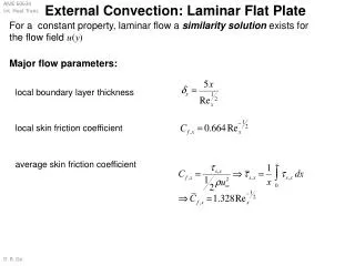
18. Laminar Velocity Boundary Layer • The velocity boundary layer thickness for laminar flow over a flat plate: • as u∞ increases, δ decreases (thinner boundary layer) • The local friction coefficient: • and the average friction coefficient over some distance x:

19. Methods to evaluate convection heat transfer • Empirical (experimental) analysis • Use experimental measurements in a controlled lab setting to correlate heat and/or mass transfer in terms of the appropriate non-dimensional parameters • Theoretical or Analytical approach • Solving of the boundary layer equations for a particular geometry. • Example: • Solve for q • Use evaluate the local Nusselt number, Nux • Compute local convection coefficient, hx • Use these (integrate) to determine the average convection coefficient over the entire surface • Exact solutions possible for simple cases. • Approximate solutions also possible using an integral method

20. Empirical method • How to set up an experimental test? • Let’s say you want to know the heat transfer rate of an airplane wing (with fuel inside) flying at steady conditions…………. • What are the parameters involved? • Velocity, –wing length, • Prandtl number, –viscosity, • Nusselt number, • Which of these can we control easily? • Looking for the relation:Experience has shown the following relation works well:

21. L insulation Experimental test setup • Measure current (hence heat transfer) with various fluids and test conditions for • Fluid properties are typically evaluated at the mean film temperature

23. Similarity Variables

24. Laminar Thermal Boundary Layer: Blasius Similarity Solution Boundary conditions:

25. Similarity Direction h Direction of similarity

26. This differential equation can be solved by numerical integration. One important consequence of this solution is that, for pr >0.6: Local convection heat transfer coefficient:

27. Local Nusselt number:

28. Average heat transfer coefficient:

29. y x y x For large Pr (oils): For small Pr (liquid metals): Pr > 1000 Pr < 0.1 Fluid viscosity less than thermal diffusivity Fluid viscosity greater than thermal diffusivity

30. A single correlation, which applies for all Prandtl numbers, Has been developed by Churchill and Ozoe..

31. Transition to Turbulence • When the boundary layer changes from a laminar flow to a turbulent flow it is referred to as transition. • At a certain distance away from the leading edge, the flow begins to swirl and various layers of flow mix violently with each other. • This violent mixing of the various layers, it signals that a transition from the smooth laminar flow near the edge to the turbulent flow away from the edge has occurred.

32. Flat Plate Boundary Layer Trasition • Important point: • Typically a turbulent boundary layer is preceded by a laminar boundary layer first upstream •  need to consider case with mixed boundary layer conditions!

33. Turbulent Flow Regime • For a flat place boundary layer becomes turbulent at Rex ~ 5 X 105. • The local friction coefficient is well correlated by an expression of the form Local Nusselt number:

34. Mixed Boundary Layer • In a flow past a long flat plate initially, the boundary layer will be laminar and then it will become turbulent. • The distance at which this transitions starts is called critical distance (Xc) measured from edge and corresponding Reynolds number is called as Critical Reynolds number. • If the length of the plate (L) is such that 0.95  Xc/L  1, the entire flow is approximated as laminar. • When the transition occurs sufficiently upstream of the trailing edge, Xc/L  0.95, the surface average coefficients will be influenced by both laminar and turbulent boundary layers.

35. Leading Edge Trailing Edge Xc L

36. On integration: For a smooth flat plate: Rexc = 5 X 105

37. For very large flat plates: L >> Xc, in general for ReL > 108

38. Cylinder in Cross Flow

42. Cylinder in Cross Flow

43. Smooth circular cylinder where Valid over the ranges 10 < Rel < 107 and 0.6 < Pr < 1000

45. Array of Cylinders in Cross Flow • The equivalent diameter is calculated as four times the net flow area as layout on the tube bank (for any pitch layout) divided by the wetted perimeter.

46. For square pitch: For triangular pitch:

47. Number of tube centre lines in a Shell: Dsis the inner diameter of the shell. Flow area associated with each tube bundle between baffles is: where A s is the bundle cross flow area, Ds is the inner diameter of the shell, C is the clearance between adjacent tubes, and B is the baffle spacing.

48. the tube clearance C is expressed as: Then the shell-side mass velocity is found with Shell side Reynolds Number:

49. Shell-Side Heat Transfer Coefficient