Download
1 / 36
360 likes | 370 Views
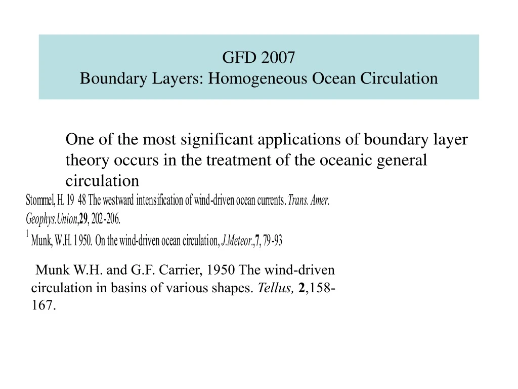
GFD 2007 Boundary Layers: Homogeneous Ocean Circulation. One of the most significant applications of boundary layer theory occurs in the treatment of the oceanic general circulation. Munk W.H. and G.F. Carrier, 1950 The wind-driven circulation in basins of various shapes. Tellus, 2 ,158-167.

E N D
GFD 2007Boundary Layers: Homogeneous Ocean Circulation One of the most significant applications of boundary layer theory occurs in the treatment of the oceanic general circulation Munk W.H. and G.F. Carrier, 1950 The wind-driven circulation in basins of various shapes. Tellus, 2,158-167.
Henry Stommel Holly Pedlosky
The homogeneous model f/2 Simplest model = constant H z y x hb
The model Upper Ekman layer provides a pumping z = H+hb z = hb fo =2 sin y z plane R
Model equations of motion (1) Vorticity equation Integrating vertically, Geostrophic stream function
Equations of motion (2) and scaling U , L for velocity and length, UL for L)-1 or time. Choose U as Ekman pumping scales with
Governing equation and boundary layer scales Inertial scale Munk Stommel Relative strength of bottom topography to effect
The singular perturbation problem and S are all small. Boundary layer scales are much less than the full basin width. They multiply the higher order derivatives. y =1 L is the north-south extent of the basin. x =0, y =0 x =xe
The interior problem For a flat bottom interior, when all the boundary layer scales are small, the governing equation is : Sverdrup relation. 1st order ode in x alone. Only determines interior meridional velocity. Can’t satisfy no slip and can satisfy no normal flow, or =0, only on one boundary, east or west but not both.
Two possible (at least) interior solutions 1)Satisfy =0 on western boundary or 2) on eastern boundary example x
An Integral constraint (1) C C a steady (closed ) streamline. = 0
An Integral Constraint (2) The net input of vorticity on each streamline must be balanced by bottom friction and lateral friction (for steady flow) If there are eddies that flux vorticity integral must include that effect. but this last term must be zero for the streamline coincident with boundary.
The Energy constraint Multiplying by and integrating over the closed basin for steady flow: So that and we must be negatively correlated. On the whole this implies a circulation in the direction of the wind stress.
The linear boundary layer problem For a flat bottom, linear eqn. becomes . and interior solution is
The Stommel model In the boundary layer, keeping only x derivatives and letting After a single integration in x Consider case Ignore term c (this is a singular perturbation) to obtain Stommel’s model of the boundary layer.
The Stommel solution To satisfy no normal flow condition on x =0 If we try to do the same on the eastern boundary bl correction function grows exponentially. No boundary layer possible on eastern boundary. Hence,y) =0 in interior solution s=fL
The western intensification Stommel’s original explanation of western intensification and the existence of the Gulf Stream due to effect. Controlled by boundary layer
The no slip condition and the sublayer • Need to satisfy no slip condition .So far ignored. • The vorticity balance of the whole basin depends on the lateral diffusion term if no slip condition applies. So far ignored. To preserve the total order of the system and to satisfy the no slip condition we need to include terms b and c in boundary layer equation. Now, x= s For sub layer define
Correction function in sublayer Essentially, the Stewartson E1/4 layer. Independent of , symmetric east west. matching
The dissipation balance (1) Integrate across basin. Ignore y derivatives in dissipation terms. For Ekman pumping independent of x, =0 for no slip Boundary current has no net vorticity The contribution of the sublayer to the final term is: Balances input of vorticity
The dissipation balance (2) Most of the fluid flowing south in the interior returns in the Stommel layer and not the sublayer. On those streamlines always outside the sublayer the dissipation balance only involves bottom friction, Integrating across the basin from just outside the sublayer to the eastern boundary, the total mass flux balances and: Vorticity balance on streamlines through Stommel layer
An integral balance for the boundary layer y2 y1 R Ignoring vorticity input by wind in the boundary layer region x = 0
The integral balance with bl approximations used If the bottom is flat and the no slip condition applies the vorticity put into the fluid along latitude y must be dissipated in the boundary layer at that latitude to obtain a steady state balance. In the presence of an uneven bottom the pressure drag can locally enter the balance but when integrated along a closed streamline the topographic term can give no net contribution (just as the planetary or relative vorticity advection)
See Hughes C. W. and B. de Cuevos. 2001 Why western boundary currents in realistic oceans are inviscid: A link between form stress and bottom pressure torques. J.Phys. Ocean.31, 2871-2885.
Inertial boundary layers Most fluid will go through inertial layer but there is not enough dissipation in the layer to satisfy the vorticity balance on those streamlines Total vorticity conserved on streamline
Inertial boundary layer:Example I U = constant Far from the boundary the relative vorticity is negligible so Q( y y On all streamlines connected to far field Q(
Inertial layer (2) In non-dimensionless units Interior flow needs to be westward. Can’t close circulation or satisfy no slip. Greenspan H.P. 1962 A criterion for the existence of inertial boundary layers in the oceanic circulation. Proc. Nat. Acad.Sci,, 48, 2034-2039. Pedlosky, J. 1965 A note on the western intensification of the oceanic circulation. J. Marine Res. , 23, 207-209.
Inertial sublayer vorticity flux through sublayer could balance vorticity input by the wind. Most streamlines don’t go through sublayer. In Stommel model the streamlines that did not go through the sublayer still had a proper vorticity balance. This is no longer true. Boundary layer Reynolds number Inertial/viscous in inertial layer >> 1 What happens?
Inertial Runaway Panel a shows the linear solution when I is zero, panel b shows the case for Re=1, panel c shows the flow for Re = 1.95 , while for panel d, Re=4.29, Circulation intensifies until vorticity is dissipated on each streamline.
References Veronis, G. 1966 Wind-driven ocean circulation-part I. Linear theory and perturbation analysis. Deep-Sea Res.13, 17-29 Ierley, G.R. and V.A. Sheremet. 1995 Multiple solutions and advection-dominated flows in the wind-driven circulation. Part I: Slip. J. Marne Res.53, 703-737, Fox-Kemper, B. 2003. Eddies and Friction: Removal of vorticity from the wind-driven gyre. MIT/WHOI Joint Program Ph.D. thesis Fox-Kemper,B. and J.Pedlosky, 2004. Wind-driven barotropic gyre I: Circulation control by eddy vorticity fluxes to an enhanced removal region. J. Marine Res., 62, 169-193.
The enhanced sublayer When we set a value of A, the momentum mixing coefficient, we are conflating two somewhat independent physical processes. The first is a measure of the unresolved eddy scales and their effect on the large scale flow in the interior and the boundary layers. The second is a measure of the strength of the interaction of the fluid with the boundary. Decreasing the single parameter, A, then reduces both processes. If the interaction with the boundary is related to a different physical process than the dissipation of vorticity away from the boundary, it seems overly constraining to represent both with a single parameterization. Fox-Kemper allowed the dissipation to locally increase in a sublayer near the western boundary.
The enhanced sublayer (2) Near the boundary variable
The turbulent boundary layer and the role of eddies. For substantial values of the interior Reynolds numbers the western boundary layer becomes unstable to shear instability. The eddies in the inertial portion of the boundary layer, through which most of the mean streamlines pass, will flux vorticity to the sublayer where it is dissipated by the locally enhanced friction. The process is a three step one, instability, flux and dissipation and the student is referred to Fox-Kemper and Pedlosky for the details of the analysis. The result though is striking and shown in the following figure.
The arrested runaway compare Control of large scale circulation by details of dissipation in the boundary layer.