Download
1 / 28
280 likes | 464 Views
DISTRIBUTED RAINFALL RUNOFF MODELS APPLIED TO THE DARGLE. Prof. Eng. Ezio TODINI e-mail : todini@geomin.unibo.it. Rainfall Runoff Models. Black Box M. Semi Distributed M. Distributed M. DISTRIBUTED RAINFALL-RUNOFF MODELLING. Advantages of Distributed Models

E N D
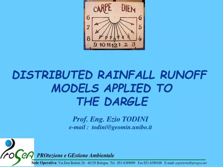
DISTRIBUTED RAINFALL RUNOFF MODELS APPLIED TO THE DARGLE Prof. Eng. Ezio TODINI e-mail : todini@geomin.unibo.it
Rainfall Runoff Models Black Box M. Semi Distributed M. Distributed M. DISTRIBUTED RAINFALL-RUNOFF MODELLING • Advantages of Distributed Models • Physical meaning of model parameters • Distributed representation of phenomena Limited calibration requirements Possibility of internal analysis
Model 1: AFFDEF Mass Balance in each cell • Main model characteristics: • Modified CN for estimating infiltration • Radiation method for evapotranspiration • Muskingum-Cunge for ovrland and channel flow
Model 2: TOPKAPI • Main model characteristics • Vertical lumping of hydraulic conductivity • Dunne infiltration • Soil horizontal flow, overland and channel flows represented using a kinematic equation • Horizontal lumping of kinematic equations Model for the single cell
ODE TOPKAPI Distributed approachThe model for the single cell SOIL COMPONENT mass conservation moment conservation
ODE TOPKAPI Distributed approachThe model for the single cell SURFACE COMPONENT mass conservation moment conservation …
ODE TOPKAPI Distributed approachThe model for the single cell CHANNEL COMPONENT mass conservation moment conservation …
Model 3: MIKE SHE • Main model characteristics: • 1D Richards equations for unsaturated zone • 3D Boussinesq equation for greoundwater • Parabolic approximation for overland flow
Case study The Dargle Republic of Eireland County of Wicklow
Case study • - Surface Area circa 122 km2 • Elevation from 20 m to 713 m a.s.l. • Sandy and sandy loam for about • 1.5 m
Dunne Saturation mechanism Horton The “unrealistic” profile used in MIKE SHE to meet the observations
Efficiency Coefficients Variance of obs. = 17.85 Variance of errors= 6.97 Nash Sutcliffe= 0.59 Explained Variance= 0.61 Coefficient of correlation =0.91 Volume Control = 0.74 Willmott= 0.93 Results: AFFDEF
Efficiency Coefficients Variance of obs. = 17.85 Variance of errors= 6.97 Nash Sutcliffe= 0.59 Explained Variance= 0.61 Coefficient of correlation =0.91 Volume Control = 0.74 Willmott= 0.93 5 [Km2 ] Areal threshold Risults: AFFDEF Average computer time = 5 min 0.01 [ms-1] Saturated Hydraulic Conductivity Infiltration Res. Const 4320000[s] Infiltration constant 0.7 Infiltration Capacity 0.1 Uniform value for curve number: 20
Efficiency Coefficients Variance of obs. = 17.85 Variance of errors= 4.01 Nash Sutcliffe= 0.77 Explained Variance= 0.77 Coefficient of correlation =0.91 Volume Control = 0.90 Willmott= 0.95 Results: TOPKAPI
Efficiency Coefficients Variance of obs. = 17.85 Variance of errors= 4.01 Nash Sutcliffe= 0.77 Explained Variance= 0.77 Coefficient of correlation =0.91 Volume Control = 0.90 Willmott= 0.95 Results: TOPKAPI Average comp. time = 5 min
Efficiency Coefficients Variance of obs. = 17.85 Variance of errors= 8.32 Nash Sutcliffe= 0.52 Explained Variance= 0.54 Coefficient of correlation =0.85 Volume Control = 0.80 Willmott= 0.90 Results: MIKE SHE
Efficiency Coefficients Variance of obs. = 17.85 Variance of errors= 8.32 Nash Sutcliffe= 0.52 Explained Variance= 0.54 Coefficient of correlation =0.85 Volume Control = 0.80 Willmott= 0.90 Results: MIKE SHE Average computer time = 2.5 h
Distributed soil moisture Saturation percentage
Ponte Spessa Example of link ECMWF -TOPKAPI on the Po Basin The basin closed at Ponte Spessa (Surface area 36,900 km2 )
The Soil Types The Land Uses The DEM