Download
1 / 26
1.09k likes | 3.73k Views
Rainfall-Runoff Relationships. Overview. Hydrologic Cycle Design storms Precipitation Amount estimation Distribution Abstraction Runoff Estimation methods Terminology. Hydrologic Cycle. Precipitation Abstraction Canopy storage Surface storage Infiltration Evapotranspiration

E N D
Overview • Hydrologic Cycle • Design storms • Precipitation • Amount estimation • Distribution • Abstraction • Runoff • Estimation methods • Terminology
Hydrologic Cycle • Precipitation • Abstraction • Canopy storage • Surface storage • Infiltration • Evapotranspiration • Runoff • Ground water flow
Design Storms • Depending on regulations, hydraulic structures are designed to handle a certain storm • Storms are classified with a return period (1yr, 2yr, 5yr, 10yr, etc.) and a duration (from 0 to 24 hrs) • Historic probability not truth • Doubling the return period does not double the rainfall amount • Short duration storms are likely more intense
Precipitation • Estimating precipitation amount • Intensity-Duration-Frequency (IDF) curves • Localized • D = i*T (equation 3.3) • D = depth • i = (K*F^x)/(T + b)^n • K, b, x, and n are constants at each location • T = duration • U.S. Weather Bureau Technical Paper NO. 40 (TP 40) • Given frequency and duration • See storms in Appendix 3A on page 477
Precipitation • Many methods for estimating rainfall distribution • Depth-Duration-Frequency (DDF) • IDF constants are needed • Normally the best fitting curve • Soil Conservation Service (SCS) rainfall pattern • Easy method • Equation 3.6 is a good estimate for both type II and III storms • Storms less than 24 hours use the steepest part of the curve (fig. 3.10) • Chicago Hyetograph • Most involved • IDF constants are needed
Abstractions • Interception • Evapotranspiration • Bank Storage • Surface Storage • Infiltration • Richards • Horton’s • Holtan’s • Green-Ampt
Infiltration • Green-Ampt • f(t) = K[y*Dq/F(t) + 1] • f(t) = infiltration rate at a given time • K = hydraulic conductivity of the wetted soil • y = pressure head for wetting at the wetting front • Dq = (1 – se)*qe = change in water content across the wetting front • se = effective saturation • qe = effective porosity • F(t) = cumulative infiltration at a given time
Runoff • Effective rainfall is the rainfall that runs off. • Runoff volume is equal to effective rainfall • SCS curve number (CN) approach • Q = (P – 0.2*S)^2/(P + 0.8*S) (equation 3.21) • Q = accumulated runoff • P = accumulated precipitation • S = 1000/CN – 10 = maximum soil water retention • CN values can be found in table 3.16 or Appendix 3C • Need to know what Hydrologic soil group the soil is in • Found in soil survey, Appendix 3B, or page 64
CN Example • Estimating runoff from a 1 ac industrial lot • Hydrologic soil group = C • CN = 91 • Antecedent moisture condition (AMC) II • 25-yr 24-hr rainfall at 7 inches • SCS type II storm • S = 1000/91 – 10 = .99 in • Q = (7 – 0.2*.99)^2/(7 + 0.8*.99) = 5.94 in • Qtotal = Q*area = 5.94 ac-in
Converting CN • Antecedent moisture condition II is the most common for calculations • If alternate (AMC I or AMC III) • CN(I) = 4.2*CN(II)/[10 – 0.058*CN(II)] • CN(III) = 23*CN(II)/[10 + 0.13*CN(II)]
Hydrograph Approach • 5 areas • 5 excess rainfalls • One rainfall excess with one area • One part of the hydrograph • Second rainfall excess with one area • Another hydrograph • Additive to the first
tl tp = tl + D/2 D tc tp Area under the curve = volume of runoff = effective rainfall qp Flow Rate tb Time Runoff Terminology
Runoff Terminology • qp = peak flow rate • tp = time to peak flow • D = duration of time increment (D usually 1/5th to 1/3rd of tp) • tl = lag time • tc = time of concentration
Peak Flow • Rational Method • qp = CiA (equation 3.70) • qp = peak flow rate (cfs) • C = dimensionless coefficient (table 3.24) • i = intensity (iph) • A = drainage area (ac) • Only works for areas with uniform rainfall (small areas)
Peak Flow • SCS-TR55 Method • qp = qu*A*Q*Fp • qp = peak flow rate (cfs) • qu = unit peak discharge (cfs/inch/square mile) • log(qu) = C0 + C1*log(tc) + C2*[log(tc)]^2 • C0, C1, C2 in table 3.26 • A = drainage area • Q = runoff in inches (24-hr storm of desired frequency) from CN method • Fp = pond and/or swamp adjustment (table 3.25)
Time of Concentration • Time of concentration is the time between the end of the rainfall excess and the point of inflection on the falling limb • Many ways to estimate including • Equation 3.47, 3.51, and 3.52 • Equation 3.52 (SCS) states that tl = 0.6tc giving tc = tl/0.6
Lag Time • Time from the center of the effective rainfall • Many ways to estimate • Equations 3.26, 3.53, and 3.54 • Equation 3.53 (SCS) states that • tl = L^.8*(S + 1)^.7/(1900*Y^.5) (in hours) • L = hydraulic length of the watershed in feet • S = maximum soil water retention • Y = average land slope in percent
Time to Peak • Almost always solved after tl • tp = tl + D/2 (equation 3.26) • Equation 3.55 can also be used • Complicated • tp is used in further calculations
Unit Hydrograph • Usually 1 inch of rainfall excess • Obtain hydrograph parameters for this setup • Peak flow for other storms is proportional to this storm • Ex: rainfall excess is 0.75 qp of the storm will be 0.75*qp of the unit hydrograph • This method is only a concept not extremely realistic
Triangular Hydrographs • A common way to represent a hydrograph is by using the peak flow and time to peak as the top of a triangle • At t = 0 the value of q is 0 • At tb the value of q is 0 • Figure 3.34shows how the different hydrographs compare
Gamma Function • When q/qp is plotted against t/tp figure 3.36 is the result • V is the area under the curve or the volume of rainfall excess
Using Hydrographs • Develop pre and post development hydrographs • Triangular for comparison • Gives a rough volume of storage needed for a reservoir • Figure 6.12 has outline
qp1 S = tb1*(qp1-qp2)/2 Flow qp2 S tb1 Time