Download
1 / 36
470 likes | 1.01k Views
Rainfall-runoff modeling. ERS 482/682 Small Watershed Hydrology. runoff (discharge). rainfall. What are models?. A model is a conceptualization of a system In hydrology, this usually involves the response of a system to an external stimuli. What are models?.

E N D
Rainfall-runoff modeling ERS 482/682 Small Watershed Hydrology
runoff (discharge) rainfall What are models? • A model is a conceptualization of a system • In hydrology, this usually involves the response of a system to an external stimuli
What are models? • A model is a conceptualization of a system • In hydrology, this usually involves the response of a system to an external stimuli • Models are tools that are part of an overall management process
Data collection Management objectives, options, constraints Make management decisions Model development and application
http://water.usgs.gov/outreach/OutReach.html Why model? • Systems are complex
Why model? • Systems are complex • If used properly, can enhance knowledge of a system • Models should be built on scientific knowledge • Models should be used as ‘tools’
Rules of modeling • RULE 1: We cannot model reality • We have to make assumptions • DOCUMENT!!!! • RULE 2: Real world has less precision than modeling
Precision vs. accuracy • Precision • Number of decimal places • Spread of repeated computations • Accuracy • Error between computed or measured value and true value error of estimate = field error + model error
The problem with precise models… we get more precision from model than is real
Q Fundamental model concepts DRIVER area topography soilsvegetationland useetc. SYSTEMREPRESENTATION RESPONSE
Mathematical equations and parameters RESPONSE DRIVER SYSTEM REPRESENTATION Basic model
The wholeworld The modelworld Figure 9-37 (Dingman 2002)
Small watershed Runoff processes to model Table 9-8 (Dingman 2002) ASSUMPTION!
usually small antecedentsoil-watercontent, 0 Effective water input, Weff • Effective (excess) rainfall • Does not include evapotranspiration or ground water storage that appears later ASSUMPTION! ASSUMPTION! where ET = event water evapotranspired during event Sc = canopy storage during event D = depression storage during event = soil-water storage during event
Estimating Weff constantfraction constantrate initialabstraction infiltrationrate Figure 9-40 (Dingman 2002)
initial abstraction Estimating Weff • SCS curve-number method where Vmax = watershed storage capacity [L] W = total rainfall [L] Figure 9-42 (Dingman 2002)
Based on land use in Table 9-12,soil group in Table 9-11, andsoil maps from NRCS Estimating Weff • SCS curve-number method where Vmax = watershed storage capacity [inches] W = total rainfall [inches]
From NRCSsoils mapsand GIS Table 9-12 58 72 30 58 Example 9-6 ConditionII CN Given: W = 4.2 in TW = 3.4 hr A = 1.24 mi2 L = 0.84 mi S = 0.08
Table 9-13 58 X 38 X 53 72 30 X 15 58 X 38 Example 9-6 ConditionI CN Given: W = 4.2 in TW = 3.4 hr A = 1.24 mi2 L = 0.84 mi S = 0.08
inches mi2 ft3 s-1 hr SCS method for peak discharge
From Table 9-9 SCS method for peak discharge
SCS method for peak discharge Example 9-7 Tc = 0.44 hr from Table 9-9 Given: W = 4.2 in TW = 3.4 hr A = 1.24 mi2 L = 0.84 mi S = 0.08 Weff = 0.57 in for Condition II
proportionality coefficient Rational method Q=CIA • Assumes a proportionality between peak discharge and rainfall intensity where uR= unit-conversion factor (see footnote 7 on p. 443) CR = runoff coefficient ieff = rainfall intensity [L T-1] AD = drainage area [L2]
Apply to small(<200 ac) suburbanand urban watersheds Rational method Q=CIA • Additional assumptions: • Rainstorm of uniform intensity over entire watershed • Negligible surface storage • Tc has passed • Return period for storm is same for discharge
Rational method Q=CIA • The proportionality coefficient, CR accounts for • Antecedent conditions • Soil type • Land use • Slope • Surface and channel roughness
Rational method Q=CIA • Approach • Estimate Tc Table 9-9 • Estimate CR Table 9-10 or Table 10-9 (Dunne and Leopold 1978) • Estimate ieff for return period T • Usually use intensity-duration-frequency (IDF) curves Figure 15.1 (Viessman and Lewis 1996)
Rational method Q=CIA • Approach • Estimate Tc Table 9-9 • Estimate CR Table 9-10 or Table 10-9 (Dunne and Leopold 1978) • Estimate ieff for return period T • Usually use intensity-duration-frequency (IDF) curves • Apply equation to get qp Viessman and Lewis (1996)
Rational method vs. SCS CN method • Rational method • Small (<200 acres) urbanized watershed • Small return period (2-10 yrs) • Have localized IDF curves • SCS Curve Number method • Rural watersheds • Average soil moisture condition (Condition II)
Adaptations • Rational method • Modifications for greater return periods • Runoff coefficients for rural areas (Table 10-9: Dunne and Leopold 1978) • Modified rational method for TcTW • SCS TR-55 method • Applies to urban areas • Has a popular computer program
Adaptations • SCS TR-55 method (cont.) • Approach • Find the type of storm that applies from Figure 16.19 (Viessman and Lewis 1996) • Use CN to determine Ia from Table 15.5 (Viessman and Lewis 1996) • Calculate Ia/P • Find qu = unit peak discharge from figure for storm type in cfs mi-2 in-1 (Viessman and Lewis 1996) • Find runoff Q in inches from Figure 10-8 (Dunne and Leopold 1978) for P • Find peak discharge for watershed as Qp = quQA
Qef Unit hydrograph • Definition: hydrograph due to unit volume of storm runoff generated by a storm of uniform effective intensity occurring within a specified period of time uniform intensityover TW 1 unit Multiply unit hydrographby Weff to get stormhydrograph Assumption: Weff = Qef
Unit hydrograph development Figure 9-45 • Choose several hydrographs from storms of same duration (~X hours) (usually most common/critical duration) • For each storm, determine Weff and plot the event flow hydrograph for each storm • For each storm, multiply the ordinates on the hydrograph by Weff-1 to get a unit hydrograph • Plot all of the unit hydrographs on the same graph with the same start time • Average the peak values for all of the unit hydrographs, and the average time to peak for all of the hydrographs • Sketch composite unit graph to an avg shape of all the graphs • Measure the area under the curve and adjust curve until area is ~1 unit (in or cm) of runoff End result: X-hr unit hydrograph
Unit hydrograph application • Multiply unit hydrograph by storm size • Add successive X-hour unit hydrographs to get hydrographs of successive storms (Figures 9-46 and 9-47)
Unit hydrograph • Predicts flood peaks within ±25% • Need only a short period of record • Can apply to ungauged basins by regionalizing the hydrograph • Synthetic unit hydrographs
Synthetic unit hydrograph • Unit hydrograph for ungauged watershed derived from gauged watershed • Example (Dingman 2002): • Example (Dunne and Leopold 1978): where Ct = coefficient (1.8-2.2) L = length of mainstream from outlet to divide (miles) Lc = distance from outlet to point on stream nearest centroid (miles) Cp = coefficient (370-440) Tb = duration of the hydrograph (hrs)
-index Figure 8-7 (Linsley et al. 1982) Figure 10-7 (Dunne & Leopold 1978)