Download
1 / 53
3.02k likes | 6.6k Views
Introduction to Computational Fluid Dynamics Lecture 5: Discretization, Finite Volume Methods. Transport Equations. Mass conservation The integral form of mass conservation equation is where ρ is the density in domain Ω , v the velocity of the fluid and n the unit normal to the boundary, S. .

E N D
Introduction to Computational Fluid DynamicsLecture 5: Discretization, Finite Volume Methods
Transport Equations • Mass conservation The integral form of mass conservation equation is where ρ is the density in domain Ω , v the velocity of the fluid and n the unit normal to the boundary, S.
Transport Equations • Momentum Conservation T = Stress tensor, n = normal to the boundary b = body force (gravity, centrifugal, Coriolis, Lorentz etc..)
Transport Equations • Energy transport T = temperature, k = thermal conductivity, c = specific heat at constant pressure, Q = heat flux (Species transport is similar – no specific heat term)
Finite Volume Methods • See class slides for finite volume methods
Discretization Courtesy: Fluent, Inc.
Overview • The Task • Why discretization? • Discretization Methods • Dealing with Convection and Diffusion • Discretization Errors Courtesy: Fluent, Inc.
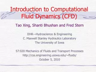
The Task • The Navier-Stokes equations equations governing the motion of fluid, in this instance, around a vehicle, are highly non-linear, second order partial differential equations (PDE’s) • Exact solutions only exist for a small class of simple flows, e.g., laminar flow past a flat plate • A numerical solution of a PDE or system of PDE’s consists of a set of numbers from which the distribution of the variable fcan be obtained from the set • The variable f is determined at a finite number of locations known as grid points or cells. This number can be large or small Courtesy: Fluent, Inc.
What is discretization? • Discretization is the method of approximating the differential equations by a system of algebraic equations for the variables at some set of discrete locations in space and time • The discrete locations are grid/meshpoints or cells • The continuous information from the exact solution of PDE’s is replaced with discrete values Pipe discretized into cells Courtesy: Fluent, Inc.
Discretizing the domain • Transforming the physical model into a form in which the equations governing the flow physics can be solved can be referred to as discretizing the domain Illustration of the cells Discretized domain Continuous domain Courtesy: Fluent, Inc.
Solving the PDE’s • The are a number of methods for the solution of the governing PDE’s on the discretized domain • The most important discretization methods are: • Finite Difference Method (FDM) • Finite Volume Method (FVM) • Finite Element Method (FEM) Courtesy: Fluent, Inc.
Finite Difference Method - Introduction • Oldest method for the numerical solution of PDE’s • Procedure: • Start with the conservation equation in differential form • Solution domain is covered by grid • Approximate the differential equation at each grid point by approximating the partial derivatives from the nodal values of the function giving one algebraic equation per grid point • Solve the resulting algebraic equations for the whole grid. At each grid point you solve for the unknown variable value and the value of it’s neighboring grid points Courtesy: Fluent, Inc.
ui-1 ui ui+1 Dx Dx Finite Difference Method - Concept • The finite difference method is based on the Taylor series expansion about a point, x Subtracting the two eqns above gives Adding the two eqns above gives Courtesy: Fluent, Inc.
Finite Difference Method - Application • Consider the steady 1-dimensional convection/diffusionequation: • From the Taylor series expansion, get Courtesy: Fluent, Inc.
Finite Difference Method - Algebraic form of PDE • Substitute the discrete forms of the differentials to get: Algebraic form of PDE Courtesy: Fluent, Inc.
Finite Difference Method - Summary • Discretized the one-dimensional convection/diffusion equation • The derivatives were determined from a Taylor series expansion • Advantages of FDM: simple and effective on structured grids • Disadvantages of FDM: conservation is not enforced unless with special treatment, restricted to simple geometries Courtesy: Fluent, Inc.
Boundary node Control volume Computational node Finite Volume Method - Introduction • Using Finite Volume Method, the solution domain is subdivided into a finite number of small control volumes by a grid • The grid defines to boundaries of the control volumes while the computational node lies at the center of the control volume • The advantage of FVM is that the integral conservation is satisfied exactly over the control volume Courtesy: Fluent, Inc.
N NE NW n E P W e w Dy s S SE SW Dx dxw dxe j i Finite Volume Method - Typical Control Volume • The net flux through the control volume boundary is the sum of integrals over the four control volume faces (six in 3D). The control volumes do not overlap • The value of the integrand is not available at the control volume faces and is determined by interpolation Courtesy: Fluent, Inc.
j i Finite Volume Method - Application • Consider the one-dimensional convection/diffusion equation • The finite volume method (FVM) uses the integral form of the conservation equations over the control volume: • Integrating the above equation in the x-direction across faces e and w of the control volume and leaving out the source term gives • The values of f at the faces e and w are needed N n E P W e w s S Courtesy: Fluent, Inc.
Finite Volume Method - Interpolation • Using a piecewise-linear interpolation between control volume centers gives } • linear interpolation between nodes • face is midway between nodes • equivalent to Central Difference Scheme (CDS) where • Under assumption of continuity, discrete form of PDE from FVM is identical to FDM Courtesy: Fluent, Inc.
fL -Pe >> 1 Pe = -1 Pe = 0 Pe = 1 Pe >> 1 fo 0 L Finite Volume Method - Exact Solution • Exact solution with boundary conditions: • f = fo at x = 0, f = fL at x = L • Peclet number, Pe, is the ratio of the strengths of convection and diffusion • When the Peclet number is high (positive or negative), the profile is highly non-linear • The Central-Difference Scheme relies on a linear interpolation which will fail to capture the gradient changes in the variable f Courtesy: Fluent, Inc.
Finite Volume Method - Interpolation • The piecewise-linear or CDS interpolation may give rise to numerical errors (oscillatory or checkerboard solutions). CDS was used only as an example of discretization and is inappropriate for most convection/diffusion flows • A large number of interpolation techniques in FLUENT software that are improvements on the CDS. Some of these, in increasing level of accuracy, are: • First-Order Upwind Scheme • Power Law Scheme • Second-Order Upwind Scheme • Higher Order • Blended Second-Order Upwind/Central Difference • Quadratic Upwind Interpolation (QUICK) Courtesy: Fluent, Inc.
Sources of Numerical Errors - FDM & FVM • Discretization Errors from inexact interpolation of nonlinear profile (FVM) • Truncation Errors due to exclusion of Higher Order Terms (FDM) • Domain discretization not well resolved to capture flow physics • Artificial or False Diffusion due to interpolation method and grid Courtesy: Fluent, Inc.
Hot fluid T = 100ºC Cold fluid T = 0ºC False Diffusion (1) • False diffusion is numerically introduced diffusion and arises in convection dominant flows, i.e., high Pe number flows • Consider the problem below: • If there is no false diffusion, the temperature along the diagonal will be 100ºC • False diffusion will occur due to the oblique flow direction and non-zero gradient of temperature in the direction normal to the flow • Grid refinement coupled with a higher-order interpolation scheme will minimize the false diffusion Diffusion set to zero k=0 Courtesy: Fluent, Inc.
False Diffusion (2) Second-order Upwind First-order Upwind 8 x 8 64 x 64 Courtesy: Fluent, Inc.
Finite Volume Method - Summary • The FVM uses the integral conservation equation applied to control volumes which subdivide the solution domain, and to the entire solution domain • The variable values at the faces of the control volume are determined by interpolation. False diffusion can arise depending on the choice of interpolation scheme • The grid must be refined to reduce “smearing” of the solution as shown in the last example • Advantages of FVM: Integral conservation is exactly satisfied, Not limited to grid type (structured or unstructured, cartesian or body-fitted) Courtesy: Fluent, Inc.
Finite Element Method - Introduction • Using Finite Element Method, the solution domain is subdivided into a finite number of small elements by a grid • The grid defines to boundaries of the elements and location of nodes — for higher-order elements, there can be mid-side nodes also • FEM uses multi-dimensional shape functions which afford geometric flexibility and limit false diffusion Mid-side node Finite element Computational node Courtesy: Fluent, Inc.
Finite Element Method - Typical Element • 9-noded quadrilateral • Within each element, the velocity and pressure fields are approximated by: where ui, vi, pi are the nodal point unknowns and fi and yi are interpolation functions • Quadratic approximation for velocity, linear approximation for pressure required to avoid spurious pressure modes nodes with u, v, p nodes with u, v Courtesy: Fluent, Inc.
Finite Element Method - Interpolation • The solution on an element is represented as: fi where N are the basis functions. We choose basis functions that are 1 at one node of the element and 0 at all other the nodes. fi+1 node Courtesy: Fluent, Inc.
Finite Element Method - Application • Recall the one-dimensional convection/diffusion equation • Most often, the finite element method (FEM) uses the Method of Weighted Residuals to discretize the equation • Multiply governing equation by weight function Wiand integrate over the element • How do we choose the Wi? For Galerkin FEM, replace Wi by Ni, the shape or basis functions Courtesy: Fluent, Inc.
Finite Element Method - “Weak” form • Use integration by parts to obtain the “weak” formulation — involves first derivatives rather than second derivatives • We can now substitute the interpolation function for f: and evaluate the required integrals to produce the discrete equation: Courtesy: Fluent, Inc.
Finite Element Method - Wiggles (1) • Wiggles occur in FEM when linear weighting functions are used • Typical cures are: • Petrov-Galerkin method: where the weighting function is different from the shape function. The weighting function is asymmetric, being skewed in the direction of the upwind element Wi u Ni i-1 i i+1 Courtesy: Fluent, Inc.
Finite Element Method - Wiggles (2) • Artificial tensor viscosity: • the viscosity in the streamline direction is augmented • this is equivalent to skewing the weighting of the convection terms towards the upstream direction flow shapes of Galerkin and Streamline Upwind weighting functions for nodal point C D U C Courtesy: Fluent, Inc.
Finite Element Method - Summary • FEM solves the “weak” form of the governing equations • weak form requires continuity of lower order operators only • very similar to using the divergence theorem in FVM • The technique is conservative in a weighted sense • The weight functions an easily be made multi-dimensional • this limits false diffusion Courtesy: Fluent, Inc.
Summary • The concept of discretization was introduced. The three main methods of discretization, FDM, FVM, and FEM were detailed. • The one-dimensional convection/diffusion was used to illustrate the different methods of discretizing the partial differential equations into algebraic equations. • The process of discretization was shown to introduce errors (though minimal in some cases) through truncation of higher order terms (FDM), approximation of the integrals (FVM). • The correct interpolation of the convective fluxes across the cell faces minimizes errors in both discretization methods. Courtesy: Fluent, Inc.
Designing Grids for CFD Courtesy: Fluent, Inc.
Outline • Why is a grid needed? • Element types • Grid types • Grid design guidelines • Geometry • Solution adaption • Grid import Courtesy: Fluent, Inc.
Why is a grid needed? • The grid: • designates the cells or elements on which the flow is solved • is a discrete representation of the geometry of the problem • has cells grouped into boundary zones — where b.c.’s are applied • The grid has a significant impact on: • rate of convergence (or even lack of convergence) • solution accuracy • CPU time required Courtesy: Fluent, Inc.
Element Types • Many different cell/element and grid types are available — choice depends on the problem and the solver capabilities • Cell or element types • 2D: • 3D: 2D prism (quadrilateral or “quad”) triangle (“tri”) prism with quadrilateral base (hexahedron or “hex”) tetrahedron(“tet”) prism with triangular base (wedge) pyramid Courtesy: Fluent, Inc.
Grid Types (1) • Single-block, structured grid • i,j,k indexing to locate neighboring cells • grid lines must pass all through domain • Obviously can’t be used for very complicated geometries Courtesy: Fluent, Inc.
Grid Types (2) • Multi-block, structured grid • uses i,j,k indexing with each block of mesh • grid can be made up of (somewhat) arbitrarily-connected blocks • More flexible than single block, but still limited cross-section: Courtesy: Fluent, Inc.
Grid Types (3) • Unstructured grid • tri or tet cells arranged in arbitrary fashion • no grid index, no constraints on cell layout • There is some memory/CPU overhead for unstructured referencing CFD stands for Cow Fluid Dynamics! Courtesy: Fluent, Inc.
Grid Types (4) • Hybrid grid • use the most appropriate cell type in any combination • triangles and quadrilaterals in 2D • tetrahedra, prisms and pyramids in 3D • can be non-conformal: grids lines don’t need to match at block boundaries prism layer efficiently resolves boundary layer tetrahedral volume mesh is generated automatically triangular surface mesh on car body is quick and easy to create non-conformal interface Courtesy: Fluent, Inc.
optimal (equilateral) cell circumcircle actual cell Grid Design Guidelines: Quality (1) • Quality: cells/elements are not highly skewed • Two methods for determining skewness: 1. Based on the equilateral volume: • Skewness = • Applies only to triangles and tetrahedra Courtesy: Fluent, Inc.
Grid Design Guidelines: Quality (1) 2. Based on the deviation from a normalized equilateral angle: • Skewness (for a quad) = • Applies to all cell and face shapes • High skewness values inaccurate solutions & slow convergence • Keep maximum skewness of volume mesh < 0.95 • Possible classification based on skewness: Courtesy: Fluent, Inc.
Grid Design Guidelines: Resolution • Pertinent flow features should be adequately resolved • Cell aspect ratio (width/height) should be near 1 where flow is multi-dimensional • Quad/hex cells can be stretched where flow is fully-developed and essentially one-dimensional flow inadequate better OK! Courtesy: Fluent, Inc.
Grid Design Guidelines: Smoothness • Change in cell/element size should be gradual (smooth) • Ideally, the maximum change in grid spacing should be 20%: smooth change in cell size sudden change in cell size — AVOID! • • • Dxi Dxi+1 Courtesy: Fluent, Inc.
Grid Design Guidelines: Total Cell Count • More cells can give higher accuracy — downside is increased memory and CPU time • To keep cell count down: • use a non-uniform grid to cluster cells only where they’re needed • use solution adaption to further refine only selected areas Courtesy: Fluent, Inc.
Geometry • The starting point for all problems is a “geometry” • The geometry describes the shape of the problem to be analyzed • Can consist of volumes, faces (surfaces), edges (curves) and vertices (points). Geometry can be very simple... … or more complex geometry for a “cube” Courtesy: Fluent, Inc.
Geometry Creation • A good preprocessor provides tools for creating and modifying geometry. • Geometry can also be imported from other CAD programs. • Various file types exist: • IGES • ACIS • STL • STEP • DXF • various proprietary (Universal files, etc.) Courtesy: Fluent, Inc.