Download
1 / 44
440 likes | 530 Views
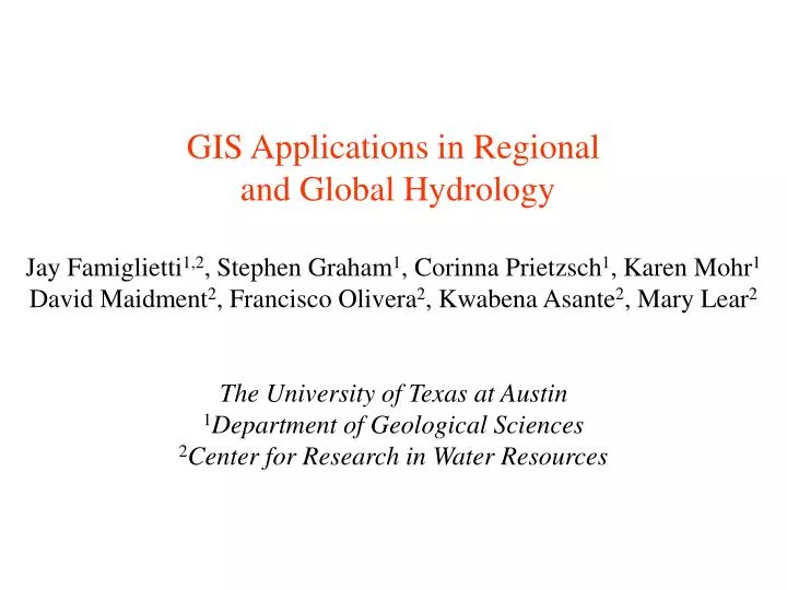
GIS Applications in Regional and Global Hydrology Jay Famiglietti 1,2 , Stephen Graham 1 , Corinna Prietzsch 1 , Karen Mohr 1 David Maidment 2 , Francisco Olivera 2 , Kwabena Asante 2 , Mary Lear 2 The University of Texas at Austin 1 Department of Geological Sciences

E N D
GIS Applications in Regional and Global Hydrology Jay Famiglietti1,2, Stephen Graham1, Corinna Prietzsch1, Karen Mohr1 David Maidment2, Francisco Olivera2, Kwabena Asante2, Mary Lear2 The University of Texas at Austin 1Department of Geological Sciences 2Center for Research in Water Resources
Overview Introduction: Jay Famiglietti GIS-Based Global-Scale Runoff Routing: Jay Famiglietti GIS Data Layers for Global Hydrologic and Climate System Modeling: Stephen Graham GIS in Remote Sensing: Corinna Prietzsch GIS Data Layers for a Regional Hydrologic and Land-Atmosphere Interaction Study: Karen Mohr
American Geophysical Union1998 Fall MeetingDecember 6, 1998Paper Number: H71D-11 DTM-Based Model forGlobal-Scale Runoff Routing Francisco OliveraJames FamigliettiKwabena AsanteDavid Maidment Center for Research in Water Resources University of Texas at Austin
Runoffon the land Streamflow into the ocean Motivation Currently, most global climate models (GCM’s) ... • … do not have the capability of routing runoff from the land to the ocean. • … assume runoff arrives at the ocean instantaneously, as if flow velocities were infinite (NCAR fully-coupled land-ocean-atmosphere model - NCAR CSM). Is flow routing at a global scale worth it?
Goals • Determine whether runoff routing has a significant impact on coastline flows by comparing routed vs. unrouted runoff hydrographs. • Explore a new method for runoff routing that … • ... exploits the availability of high resolution global DTM’s. • … could be incorporated in a global climate model (GCM) like NCAR’s CSM.
Source-to-Sink Routing Model • Defines sources (or runoff producing units) where runoff enters the surface water system, and sinks (or runoff receiving units) where runoff leaves the surface water system. • Calculates hydrographs at the sinks by adding the contribution of all sources in the drainage area. • A response function is used to represent the motion of water from the sources to the sinks.
Sinks • A 3°x3° mesh is used to subdivide the whole globe into “square” boxes. • A total of 132 sinks were identified for the African continent (including inland catchments like theLake Chad Basin).
Drainage Area of the Sinks • The drainage area of each sink is delineated using raster-based GIS functions applied to GTOPO30. • GTOPO30 (EROS Data Center of the USGS, Sioux Falls, ND) is digital elevation data with an approximate resolution of 1 Km x 1 Km.
Land Boxes • A 0.5°x0.5° mesh is used to subdivide each drainage area into land boxes. • 0.5° land boxes allow the modeler to capture the geomorphology of the hydrologic system. • For the Congo River basin, 1379 land boxes were identified.
Runoff Boxes (T42 Data) • Runoff data has been calculated using NCAR’s CCM3.2 GCM over a 2.8125° x 2.8125° mesh (T42). • For the Congo River basin, 69 runoff boxes were identified.
Sources • Sources are obtained by intersecting: • drainage area of the sinks • land boxes • runoff boxes • Number of sources: • Congo River basin: 1954 • African continent: 19170
Flow Length to the Sinks • Flow-length is calculated for each GTOPO30 cell by using raster-based GIS functions, and then averaging the resulting values over the source area. • The flow time from a source to a sink is calculated by dividing the flow length by the (uniformly distributed) flow velocity.
Amazon River Basin MacKenzie River Basin Congo River Basin Yangtze River Basin Distance-Area Diagrams
Global Runoff According to NCAR’s CCM3.2 Global Climate Model (GCM)
Routing Algorithm For source j: tj = Lj/v For sink i: Qi = S Aj Rj(t)*uj(t) exp(-k tj) where: tj = flow time Lj = flow length v = flow velocity Qi = flow Aj = area Rj(t) = runoff time series uj(t) = response function k = loss coefficient
Amazon River MacKenzie River Congo River Yangtze River Routed vs Unrouted Hydrographs Assuming v = 0.3 m/s and k = 0 Routed Unrouted
Source-to-Sink vs. Cell-to-Cell Source-to-sink Cell-to-cell Assuming v = 0.3 m/s and k = 0
Conclusions (1) • A DTM-based methodology for global-scale flow routing has been developed. The methodology is independent of the geographic location and spatial resolution of the data. • The need for accounting for flow delay in the landscape, especially in large watersheds, became obvious after comparing routed vs. unrouted hydrographs. • Because the spatial distribution of the model parameters (e.g., flow velocity, v, and losses coefficient, k) is unknown, uniformly distributed values were assumed.
Conclusions (2) • The model takes advantage of “high” resolution terrain data and is able to produce results consistent with “low” resolution global data used for climate models. • The model produces similar results when compared to cell-to-cell routing models, but has the advantage of being independent of the terrain discretization.
Five-Minute, 1/2-Degree, and 1-Degree Data Sets of Continental Watersheds and River Networks for Use in Regional and Global Hydrologic and Climate System Modeling Studies Stephen Graham1 Jay Famiglietti1,2 David Maidment2 The University of Texas at Austin 1Department of Geological Sciences 2Center for Research in Water Resources
9 Data Layers 3 Resolutions 5-minute 1/2-degree 1-degree 1) Land/sea mask 2) Flow direction information 3) Flow accumulation information 4) River delineation 5) 55 Large watersheds 6) Internally draining regions 7) 19 large-scale drainage regions 8) 19 large-scale drainage regions extended to water bodies 9) Lake delineation Additional runoff data
The National Geophysical Data Center TerrainBase Global DTM Version 1.0 [Rowet al., 1995]
Data and Analysis Methods 1) Determination of a land/sea mask 2) Geolocation or ‘burning in’ of rivers 3) Filling of artificial depressions 4) Calculation of flow directions 5) Calculation of flow accumulations 6) Selection and delineation of rivers 7) Selection and delineation of watersheds 8) Lake Delineation
2) Geolocation or ‘burning in’ of rivers Digitized rivers from the CIA World Data Bank II are extracted and gridded. The elevations of grid cells that correspond to the gridded rivers are decreased by an appropriate amount, therefore giving an added incentive for water to follow the digitized paths. This process improves the location of rivers in flat areas, as well as mountainous areas where narrow canyons may be averaged out in the DEM.
3) Filling of artificial depressions Artificial and natural depression are both present in DEMs. In order for river channels to flow to their mouth at a water body, the course of the river must follow a monotonically decreasing path, as is defined by the flow direction grid. Consequently, sinks must be eliminated except at terminal points for water accumulation, such as inland seas. Certain sinks may also be selected to remain sinks, either manually or by using automated procedures which take into consideration such things as the depth and area of the sink. Grid: FILL elev_grid fill_grid SINK
Stream channel comparison Rivers burned into DEM and then filled Filled DEM
4,5) Calculation of flow directions and accumulations Grid: fdr_grid = FLOWDIRECTION ( fill_grid ) Grid: fac_grid = FLOWACCUMULATION ( fdr_grid )
6) Selection and delineation of rivers Grid: riv_grid = CON ( fac_grid >= 3500 , 1 )
Flow accumulation thresholds for different sized analysis regions FAC Threshold = 1000 FAC Threshold = 100
7) Selection and delineation of watersheds Create a source_grid by intersecting coasts with rivers Grid: wshed_grid = WATERSHED ( dir_grid , source_grid )
7a) Selection and delineation of internally draining areas Create a grid of the sinks that should remain sinks, which in turn are used as source cells for WATERSHED
7b) Selection and delineation of 19 global drainage regions A coast_grid can be divided into the desired sections and used as source cells for WATERSHED
7c) Extension of 19 global drainage regions to include water bodies EUCALLOCATION can be used to extend areas of the 19 regions to the oceans by assigning the closest existing value.
8) Lake Delineation Lakes are derived from CIA World Data Bank II
Changing resolutions The elevations are averaged over 1/2- and 1-degree boxes to obtain the coarser resolution 1/2- and 1-degree DEMs from the original 5-minute data. The same processes from above are then carried out at each new resolution.
Effects of Resolution 1 Coarsening of geographic features 5-minute 1/2-degree 1-degree
Effects of Resolution 2 Narrow features altered and merged with others 5-minute 1/2-degree 1-degree