WHAT IS A BOUNDARY LAYER ?

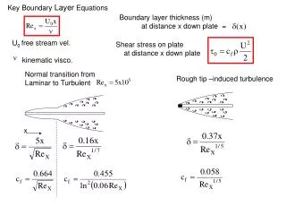
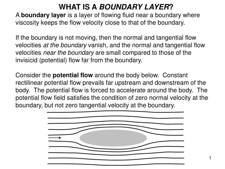
1. WHAT IS A BOUNDARY LAYER? A boundary layer is a layer of flowing fluid near a boundary where viscosity keeps the flow velocity close to that of the boundary. If the boundary is not moving, then the normal and tangential flow velocities at the boundary vanish, and the normal and tangential flow velocities near the boundary are small compared to those of the invisicid (potential) flow far from the boundary. Consider the potential flow around the body below. Constant rectilinear potential flow prevails far upstream and downstream of the body. The potential flow is forced to accelerate around the body. The potential flow field satisfies the condition of zero normal velocity at the boundary, but not zero tangential velocity at the boundary.

2. POTENTIAL FLOW AROUND THE BODY The potential flow is forced to accelerate around the body. Thus u(u/s) > 0 along a streamline near the body from near the upstream stagnation point to section A – A’. The velocity profile along the line A – A’ reflects this.

3. boundary layer BUT POTENTIAL FLOW IS NOT THE WHOLE STORY If the body is not moving, there must be some region (perhaps very thin) where the flow velocity drops to zero. This region is called a boundary layer. We will find that boundary layer thickness depends on an appropriately defined Reynolds number of the flow, and as this number gets larger the boundary layer gets thinner. Here we are interested in the case of large Reynolds number (but not so large that the flow becomes turbulent).

4. BOUNDARY-ATTACHED COORDINATES AND BOUNDARY LAYER THICKNESS Let x denotes a boundary-attached streamwise coordinate, and y denote a boundary-attached normal coordinate, as noted below. Furthermore, let (x) be defined as some measure of boundary layer thickness, i.e the thickness of the zone of retarded flow near the boundary (to be defined in more detail later). Then the boundary layer can be illustrated as follows (red line):

5. 2D NAVIER-STOKES AND CONTINUITY EQUATIONS Since the x-y coordinate system is boundary-attached, it defines a curvilinear rather than cartesian system. If the curvature is not too great, however, the governing equations for steady 2D flow around the body can be approximated as if in a cartesian coordinate system: Note that only the dynamic pressure pd is used here. The total pressure p has been decomposed as p = ph + pd,, and the static pressure ph has been cancelled out against the gravitational terms.

6. U L SCALING The scale for flow velocity in the x direction is the free-stream velocity U far from the body. The length scale in the x direction is the body length L. Boundary layer thickness (which might vary in x) is simply denoted as .

7. U L SCALING OF THE CONTINUITY EQUATION WITHIN THE BOUNDARY LAYER The continuity equation is The term u/x scales as Now consider continuity within the boundary layer. If the length scale in the direction normal to the body is denoted as  (boundary layer thickness) and the normal velocity scale is denoted as V, it follows from the estimate v/y ~ V/ and the relation that It furthermore follows that if /L << 1 then V/U << 1. Note: the sign is not important in order of magnitude estimates

8. SCALING OF THE STREAMWISE EQUATION OF MOMENTUM BALANCE WITHIN THE BOUNDARY LAYER The streamwise equation of momentum balance is Recalling from the Bernoulli equation that pd can be scaled as U2 and from the previous slide that V ~ (/L) U, the terms scale as: Note: 2u/x2 scales as U/L2, and notU2/L2. Remember why? Now multiply the scale estimates by L/U2 to get the dimensionless scale estimates for each term relative to U2/L:

9. SCALING OF THE STREAMWISE EQUATION OF MOMENTUM BALANCE contd. From the previous slide, our estimates of the terms in the streamwise momentum balance equation in the boundary layer are: where denotes the Reynolds number of the flow. The case of interest to us here is that of large Reynolds number, so that 1/Re << 1.

10. SCALING OF THE STREAMWISE EQUATION OF MOMENTUM BALANCE contd. The viscous terms in the Navier-Stokes equations are in general small compared to the other terms when the Reynolds number is large. But this cannot be true everywhere; there must be at least some small region where viscosity is powerful enough to bring the tangential velocity to zero at the boundary. The small zone where viscosity remains important even at large Reynolds number denotes the boundary layer. Thus this term can be neglected (Re <<, 1), But this term must be retained regardless of how small Re is, or there are no viscous effects anywhere. Hence the estimate

11. U L WHAT DOES THIS ESTIMATE SAY? The scale relation, or estimate says that the boundary layer  gets ever thinner compared to the length of the body L as the Reynolds number Re = (UL)/ gets large, but never goes to 0 as long as Re is finite! Outside of the boundary layer viscosity can be completely neglected in the streamwise momentum equation, and within it the streamwise momentum equation approximates as: This term is needed to bring u to 0 at the boundary!

12. SCALING OF THE NORMAL EQUATION OF MOMENTUM BALANCE WITHIN THE BOUNDARY LAYER The normal equation of momentum balance is Recalling from Bernoulli that pd can be scaled as U2, the terms scale as: Further recalling from Slide 7 that V ~ (/L)U and multiplying all terms by (/U2), the following dimensionless scale estimates are obtained:

13. SCALING OF THE NORMAL EQUATION OF MOMENTUM BALANCE contd. From the previous slide But from Slide 14, (/L) ~ (Re)-1/2, so that the estimates become or thus in the limiting approximation as Re becomes large,

14. U L WHAT DOES THIS ESTIMATE OF PRESSURE SAY? At sufficiently large Reynolds number the equation of momentum balance in the normal direction reduces to the approximation: This says that the pressure pd(x,y) can be approximated as constant in y in the boundary layer. Now let ppd(x,y) denote the dynamic pressure obtained from the potential flow (inviscid) solution. It then follows that pd(x) within the boundary layer can be obtained from ppd(x,0): Thus the solution of any boundary layer problem also requires the inviscid (potential flow) solution.

15. U L THE BOUNDARY LAYER APPROXIMATIONS OF THE NAVIER-STOKES EQUATIONS The boundary layer equations are thus: where ppdp(x) denotes the dynamic pressure obtained from the potential flow solution extrapolated to the surface of the body. The boundary conditions are so that both the tangential and normal velocities vanish on the boundary. In addition, u must approach the potential flow value as y becomes large.