Download
1 / 17
170 likes | 316 Views
Analysis of WRF Model Ensemble Forecast Skill for 80 m over Iowa. Shannon Rabideau Undergraduate Meteorology Research Symposium 12/7/2009 Mentors: Eugene Takle , Adam Deppe. Motivation. Growing wind industry Unique/ limited data for 80 m Not extrapolated from surface

E N D
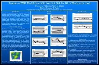
Analysis of WRF Model Ensemble Forecast Skill for 80 m over Iowa Shannon Rabideau Undergraduate Meteorology Research Symposium 12/7/2009 Mentors: Eugene Takle, Adam Deppe
Motivation • Growing wind industry • Unique/ limited data for 80 m • Not extrapolated from surface • Energy density proportional to the wind speed cubed
Data: Observed • Provided by MidAmerican Energy Corporation (MEC) • Pomeroy, IA meteorological tower • 10 min intervals, averaged hourly • “bad” data excluded • Total of 32 cases, 8 per season
Data: Forecasted • Provided by Adam Deppe • planetary boundary layer schemes • WRF: MYJ, MYNN 2.5, MYNN 3.0, Pleim, QNSE, and YSU • MM5: Blackadar • GFS and NAM initializations • Ensemble means
Data: Forecasted • 10 km grid resolution, domain of Iowa and surrounding states
Hypothesis • WRF can forecast wind speeds at 80 m with an average mean absolute error less than 2.0 m s-1for the forecast period 38-48hr (approximately 8am-6pm on day 2 of the 54hr forecast period) in all seasons with a confidence level of 95%.
Analyses • Statistical comparisons • Mean absolute error (MAE) • Bias • Root mean squared error (RMSE) • Standard deviation (STDEV) • Focus on day 2 daytime • MAE with 95% confidence interval • Over all cases and each season
Mean Absolute Error • Greater increase in MAE over time for NAM than for GFS • Ensemble mean performs best • (1.497 m s-1; 1.700 m s-1) • YSU close(+0.1 m s-1) • Blackadar(1.927 m s-1) and QNSE (2.106 m s-1) perform worst
Bias • GFS and NAM fairly comparable through the entire period • YSU has lowest avg. bias through period • (-0.130 m s-1; 0.106 m s-1) • Blackadar has highest by almost a factor of two • (-1.424 m s-1; -1.500 m s-1)
Diurnal Cycle • Schemes have more difficulty capturing nighttime speeds • 6am-6pm: average bias of -0.032 m s-1 • 6pm-6am: average bias of 0.460 m s-1 • YSU captures cycle the best • Only around 2 m s-1 between time periods
Other Results • RMSE • NAM with higher values than GFS • Ensembles perform best • MYNN schemes worst this time • STDEV • Increasing with time, more so for NAM • Ensembles with lowest values, MYNN schemes with highest
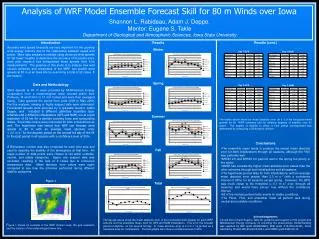
Day 2 Daytime: Seasons • Significantly better results in the spring • Missing data? Synoptic conditions? • MYNN schemes do quite well • GFS consistent through other seasons, NAM worst in summer/ fall NAM GFS
Day 2 Daytime: Schemes • Ensembles have lowest error • 1.529 m s-1 vs. 2.098 m s-1 • Blackadar (1.806 m s-1) worst - GFS • QNSE (2.421 m s-1) worst - NAM
Day 2 Daytime: Initializations • GFS less error than NAM • Averaged, 1.696 m s-1 vs. 2.294 m s-1 • GFS CI: 1.575 m s-1 to 1.817 m s-1 • NAM CI: 2.149 m s-1 to 2.440 m s-1
Conclusions • Hypothesis true for GFS over all cases, but not all seasons • CI pushes summer, fall, and winter over 2.0 m s-1 threshold (by <0.1 m s-1) • Hypothesis false for NAM over all cases and all seasons • Ensembles and YSU most accurate schemes, QNSE least accurate
References • Andersen, T. K., 2007: Climatology of surface wind speeds using a regional climate model. B.S. thesis, Dept. of Geological and Atmospheric Sciences, Iowa State University, 11 pp. • Archer, C. L., and M. Z. Jacobson, 2005: Evaluation of global wind power. J. Geophys. Res., 110, D12110. • Dudhia, J., cited 2009: WRF Physics. [Available online at http://www.mmm.ucar.edu/ wrf/users/tutorial/200909/14_ARW_Physics_ Dudhia.pdf] • Elliott, D., and M. Schwartz, 2005: Towards a wind energy climatology at advanced turbine hub-heights. Preprints, 15th Conf. on Applied Climatology, Savannah, GA, Amer. Meteor. Soc., JP1.9. • Klink, K., 2007: Atmospheric circulation effects on wind speed variability at turbine height. J. Appl. Meteorol. and Climatol., 46, 445-456. • Pryor S. C., R. J. Barthelmie, D. T. Young, E. S. Takle, R. W. Arritt, D. Flory, W. J. Gutowski Jr., A. Nunes, J. Roads, 2009: Wind speed trends over the contiguous United States. J. Geophys. Res., 114, D14105, doi: 10.1029/2008JD011416. • Takle, E. S., J. M. Brown, and W. M. Davis, 1978: Characteristics of wind and wind energy in Iowa. Iowa State J. Research., 52, 313-339. • University Corporation for Atmospheric Re-search, cited 2009: Tutorial class notes and user’s guide: MM5 Modeling System Version 3. [Available online at http://www. mmm.ucar.edu/mm5/documents/MM5_tut_Web_notes/MM5/mm5.htm] 9 • Zhang, D., and W. Zheng, 2004: Diurnal cycles of surface winds and temperatures as simulated by five boundary layer parameteriza-tions. J. Appl. Meteorol., 43, 157-169. • Wind turbine image: http://www.news.iastate.edu
Further Research • More cases without any missing data • Diurnal cycle • Synoptic conditions • Inter-annual variability • I would like to thank Eugene Takle for his guidance and support, Adam Deppe for the forecast data and other help, MEC for the observed data, and other members of Iowa State’s “wind team”.