Download
1 / 25
260 likes | 411 Views
Analysis in GIS. Analysis Components. analyses may be applied to (use as input): tabular attribute data spatial data/layers combination of spatial and tabular results may be displayed as (produce as output):

E N D
Analysis Components • analyses may be applied to (use as input): • tabular attribute data • spatial data/layers • combination of spatial and tabular • results may be displayed as (produce as output): • table subsets, table combinations, highlighted records (rows), new variables (columns) • charts • maps/map features: • highlights on existing themes • new themes/layers • combination
Availability of Analytical Capabilities:Analysis Options • Basic: Desktop GIS packages • ArcGIS ArcView • Mapinfo • Geomedia (Bentley); Geographics (Intergraph) • Advanced: Professional GIS systems • ArcGIS ArcINFO, Intergraph MGE • provide data editing plus more advanced analysis • Specialized: modelling and simulation • via scripting/programming within GIS • ArcObjects in ArcGIS • via specialized packages and/or GISs • 3-D Scientific Visualization packages • transportation planning packages • ER Mapper, PCI for raster Capabilities move ‘up the chain’ over time.
Advanced and Specialized Applications:in comparison to basic applications Most ‘basic’ analyses are used to create descriptive models of the world, that is, representations of reality as it exists. Most ‘advanced’ analysesinvolve creating a new conceptual output layer, or in some cases table(s) or chart(s), the values of which are some transformation of the values in the descriptiveinput layer. e.g. slope or aspect layer Most ‘specialized’ applications involve using GIS capabilities to create a predictive model of a real world process, that is, a model capable of reproducing processes and/or making predictions or projections as to how the world might appear.e.g. fire spread model, traffic projections
Spatial Operations centroid determination spatial measurement buffer analysis neighborhood analysis/spatial filtering geocoding polygon overlay spatial aggregation redistricting regionalization classification Attribute Operations record selection tabular via SQL ‘information clicking’ with cursor variable recoding record aggregation general statistical analysis Analysis Options: Basic
Advanced surface analysis cross section creation visibility/viewshed proximity analysis nearest neighbor layer distance matrix layer network analysis routing shortest path (2 points) traveling salesman (n points) time districting allocation Thiessen Polygon creation Specialized Remote Sensing image processing and classification raster modelling 3-D surface modelling spatial statistics/statistical modelling functionally specialized transportation modelling land use modelling hydrological modelling etc. Analysis Options: Advanced & Specialized
centroid outside polygon Spatial operations:Centroid or Mean Center • balancing point for a spatial distribution • point representation for a polygon--analogous to the mean • single point summary for a distribution (point or polygon) • useful for • summarizing change over time in a distribution (e.g Canadian pop. centroid every 10 years) • placing labels for polygons • for weird-shaped polygons, centroid may not lie within polygon
Spatial measurements: distance measures between points from point or raster to polygon or zone boundary between polygon centroids polygon area polygon perimeter polygon shape volume calculation e.g. for earth moving, resevoirs direction determination e.g. for smoke plumes Comments: possible distance metrics: straight line/airline city block/manhattan metric distance thru network time/friction thru network shape often measured by: may generate output raster: value of spatial measurement assigned to each pixel within a polygon or zone Projection affects values!!! perimeter = 1.0 for circle = 1.13 for square area x 3.54 = large number for irregular polygon Spatial operations: Spatial Measurement
Spatial operations: Spatial Measurement--example Attributes of ..... file in ArcView provides area and perimeter measurements automatically.
Buffer zones region within ‘x’ distance units buffer any object: point, line or polygon use multiple buffers at progressively greater distances to show gradation may define a ‘friction’ or ‘cost’ layer so that spread is not linear with distance Examples 200 foot buffer around property where zoning change requested 100 ft buffer from stream center line limiting development 3 mile zone beyond city boundary showing ETJ (extra territorial jurisdiction) use to define (or exclude) areas as options (e.g for retail site) or for further analysis in conjunction with ‘friction layer’, simulate spread of fire Spatial Operations:buffer zones polygon buffer point buffers line buffer
spatial convolution or filter value of each cell replaced by some function of the values of itself and the cells (or polygons) surrounding it can use ‘neighborhood’ or ‘window’ of any size 3x3 cells (8-connected) 5x5, 7x7, etc. differentially weight the cells to produce different effects kernel for 3x3 mean filter: 1/9 1/9 1/9 1/9 1/9 1/9 1/9 1/9 1/9 low frequency ( low pass) filter: mean filter cell replaced by the mean for neighborhood equivalent to weighting (mutiplying) each cell by 1/9 = .11 (in 3x3 case) smoothsthe data use larger window for greater smoothing median filter use median (middle value) instead of mean smoothing, especially if data has extreme value outliers Spatial Operations:neighborhood analysis/spatial filtering weights must sum to 1.0
combines two (or more) layers to create a third used to integrate attribute data having different spatial properties (point v. polygon) or boundaries (zip and tract) can overlay polygons on: points (point in polygon) lines (line on polygon) other polygons many different Boolean logic combinations possible Union (A or B) Intersection (A and B) A and not B ; not (A and B) Examples assign environmental samples (points) to census tracts to estimate exposure per capita (polygon on point) identify tracts traversed by freeway for study of neighborhood blight (polygon on lines) integrate census data by block with sales data by zip code (polygon on polygon) Spatial Operations:Polygon Overlay
c. a. b. Atlantic A. G. Gulf bA aA aG Spatial Matching via Polygon Overlay:example Land Use The two themes (land use & drainage basins) do not have common boundaries. GIS creates combined layer permitting calculation of land use by drainage basin. Drainage Basins cA Combined layer bG cG
Point-point • is within , e.g. find all of the customer points within 1 km of this retail store point • is nearest to , e.g. find the hazardous waste site which is nearest to this groundwater well • Point-line • ends at , e.g. find the intersection at the end of this street • is nearest to , e.g. find the road nearest to this aircraft crash site • Point-area • is contained in , e.g. find all of the customers located in this ZIP code boundary • can be seen from , e.g. determine if any of this lake can be seen from this viewpoint • Line-line • crosses , e.g. determine if this road crosses this river • comes within , e.g. find all of the roads which come within 1 km of this railroad • flows into , e.g. find out if this stream flows into this river • Line-area • crosses , e.g. find all of the soil types crossed by this railroad • borders , e.g. find out if this road forms part of the boundary of this airfield • Area-area • overlaps , e.g. identify all overlaps between types of soil on this map and types of land use on this other map • is nearest to , e.g. find the nearest lake to this forest fire • is adjacent to , e.g. find out if these two areas share a common boundary
Spatial Operations:Geocoding • assigning spatial coordinates (explict location) to addresses (implicit location) • usually assigns x,y coordinates; could be lat/long • requires street network file with street attribute information (street name and number range for each block) for all street segments (blocks) • precise matching of street names can be problemmatic • completeness (esp. for ‘new’ streets) important • PO boxes, building names, and apartment complex names cause problems.
Districting: elementary school attendance zones grouped to form junior high zones. Regionalization: census tracts grouped into neighborhoods Classification: cities categorized as central city or suburbs soils classified as igneous, sedimentary, metamorphic
Groupings may be: formal (based on in situ characteristics)e.g. city neighborhoods functional (based on flows or links): e.g. commuting zones districting/redistricting grouping contiguous polygons into districts original polygons preserved regionalization grouping polygons into contiguous regions original polygon boundaries dissolved classification grouping polygons into non-contiguous regions original boundaries usually dissolved usually ‘formal’ groupings Examples: elementary school zones to high school attendance zones (functional districting) election precincts (or city blocks) into legislative districts (formal districting) creating police precincts (funct. reg.) creating city neighborhood map (form. reg.) grouping census tracts into market segments--yuppies, nerds, etc (class.) creating soils or zoning map (class) Spatial Operations:spatial aggregation (dissolving)
Routing shortest path between two points direction instructions (locating hotel from airport) travelling salesman: shortest path connecting n points bus routing, delivery drivers Districting expand from site along network until criteria (time, distance, cost, object count) is reached; then assign area to district creating market areas, attendance zones, etc Allocation assign locations to the nearest center assign customers to pizza delivery outlets draw boundaries (lines of equidistance) based on the above market area creation example of application of Thiessen polygons Advanced Applications:Network Analysis In all cases, ‘distance’ may be measured in miles, time, cost or other ‘friction’ (e.g pipe diameter for water, sewage, etc.). Arc or node attributes (e.g one-way streets, no left turn) may also be critical.