Download

1 / 29
430 likes | 675 Views
16.2: Line Integrals 16.3: The Fundamental Theorem for Line Integrals 16.5: Curl and Divergence. 16.2. Line Integrals. Line Integrals. A Line Integral is similar to a single integral except that instead of integrating over an interval [ a , b ], we integrate over a curve C .

E N D
16.2:Line Integrals • 16.3:The Fundamental Theorem for Line Integrals • 16.5:Curl and Divergence
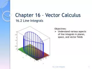
16.2 • Line Integrals
Line Integrals • A Line Integral is similar to a single integral except that instead of integrating over an interval [a, b], we integrate over a curve C. • Just as for an ordinary single integral, we can interpret the line integral of a positive function as an area. • In fact, if f (x, y) 0, Cf (x, y) ds represents the area of one side of the “fence” or “curtain”, whose base is C and whose height above the point (x, y) is f (x, y):
Line Integrals or “Curve Integrals” • Line integrals were invented in the early 19th century to solve problems involving fluid flow, forces, electricity, and magnetism. • We start with a plane curve C given by: • the parametric equations: x = x(t) y = y(t) a t b • or the vector equation: r(t) = x(t) i+ y(t) j, • and we assume that C is a smooth curve. [Meaning r is continuous and r(t)0.]
Example: • Consider the function f (x,y)= x+y and the parabola y=x2 in the x-y plane, for 0≤ x ≤2. • Imagine that we extend the parabola up to the surface f, to form a curved wall or curtain: • The base of each rectangle is the arc length along the curve: ds • The height is f above the arc length: f (x,y) • If we add up the areas of these rectangles as we move along the curve C, we get the area: Parabola is the curve C
Example (cont.’) • Next: Rewrite the function f(x,y) after parametrizing x and y: • For example in this case, we can choose parametrization: x(t)=t and y(t)=t2 • Therefore r = <t, t2> and f = t +t2 • using the fact that (recall from chapter 13! ) • ds = | r’ | dt • then ds = • And the integral becomes:
Line Integrals in 2D: • The Line integral of f along C is given by: • NOTE: • The value found for the line integral will not depend on the parametrization of the curve, provided that the curve is traversed exactly once as t increases from a to b.
Practice 1: • Evaluate C (2 + x2y) ds, where C is the upper half of the unit circle • x2 + y2 = 1. • Solution: • In order to use Formula 3, we first need parametric equations to represent C. • Recall that the unit circle can be parametrized by means of the equations • x = cos t y = sin t • and the upper half of the circle is described by the parameter interval 0t .
Practice 1 – Solution • cont’d • Therefore Formula 3 gives
Application: • If f(x, y) = 2 + x2yrepresents the density of a semicircular wire, then the integral in Example 1 would represent the mass of the wire! • The center of mass of the wire with density function is located at the point , where:
Line Integrals in 3D Space: • We now suppose that C is a smooth space curve given by the parametric equations: • x = x(t) y = y(t) z = z(t) a t b • or by a vector equation: • r(t) = x(t) i + y(t) j + z(t) k. • If f is a function of three variables that is continuous on some region containing C, then we define the line integral of f along C (with respect to arc length) in a manner similar to that for plane curves:
Line Integrals (in general) • Notice that in both 2D or 3D the compact form of writing a line integral is: • For the special case f (x, y, z) = 1, we get: • Which is simply the length of the curve C!
Example: • Evaluate C y sin zds, where C is the circular helix given by the equations: x = cos t, y = sin t, z = t, 0 t 2.
Example – Solution • Formula 9 gives:
Line Integrals of Vector Fields • Suppose that F = P i + Q j + R k is a continuous force field. • The work done by this force in moving a particle along a smooth curve C is: • Equation 12 says that work is the line integral with respect to arc length of the tangential component of the force. • This integral is often abbreviated as CF drand occurs in other areas of physics as well.
Example • Find the work done by the force field F(x, y) = x2 i – xyj • in moving a particle along the quarter-circle • r(t) = cos ti + sin tj, 0 t/2. • Solution: • Since x = cos t and y = sin t, we have • F(r(t)) = cos2t i –cos t sin t j • and r(t) = –sin t i + cos t j
Example – Solution cont’d • Therefore the work done is Anyone finds this weird or just me..?
16.3 • The Fundamental Theorem for Line Integrals
The Fundamental Theorem for Line Integrals • Recall that Part 2 of the Fundamental Theorem of Calculus can be written as: • where F is continuous on [a, b]. • This is also called: the Net Change Theorem.
The Fundamental Theorem for Line Integrals • If we think of the gradient vector f of a function f of two or three variables as a sort of derivative of f, then the following theorem can be regarded as a version of the Fundamental Theorem of Calculus:
Curl and Divergence • 16.5
Vector Field • Consider a vector function (vector field) in 3D: F = P i + Q j + R k • Meaning that there exists a potential function f, such that f =F • Recall that is the operator: • F is called a “conservative” vector field if it can be written as: F =f
Curl of a vector F • Given that: F = P i + Q j + R k and the partial derivatives of P, Q, and R all exist, then the curl of F is the vector field defined by: • Here is a better way to remember this formula! • “curl F” can also be written: XF (cross product), so we can write: • curl F is a vector!
Example 1 • If F(x, y, z) = xz i + xyz j – y2k, find curl F. • Solution:
Property of Curl: • F is called a “conservative” vector field if it can be written as:F =f • Theorem: • If f is function of three variables that has continuous second order partial derivatives, then: • curl(f) = x f = 0 • This is a great way to find out if a field F is conservative or not! • If XF = 0 then there exists a function f such that F= f, so F is conservative.
Divergence • div F is a scalar! • Property of Divergence:
Example 2 • If F(x, y, z)=xzi + xyzj +y2k, find div F. • Solution: • By the definition of divergence: • div F = F • = z + xz
Application: Maxwell’s equations • These equations describe how electric and magnetic fields are generated by charges, currents, and changes of the fields. • Maxwell first used the equations to propose that light is an electromagnetic phenomenon. • Definition of terms: