Download
1 / 50
510 likes | 727 Views
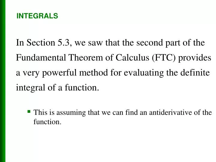
INTEGRALS. In Section 5.3, we saw that the second part of the Fundamental Theorem of Calculus (FTC) provides a very powerful method for evaluating the definite integral of a function. This is assuming that we can find an antiderivative of the function. INTEGRALS.

E N D
INTEGRALS • In Section 5.3, we saw that the second part of the Fundamental Theorem of Calculus (FTC) provides a very powerful method for evaluating the definite integral of a function. • This is assuming that we can find an antiderivative of the function.
INTEGRALS 5.4Indefinite Integrals and the Net Change Theorem • In this section, we will learn about: • Indefinite integrals and their applications.
INDEFINITE INTEGRALS AND NET CHANGE THEOREM • In this section, we: • Introduce a notation for antiderivatives. • Review the formulas for antiderivatives. • Use the formulas to evaluate definite integrals. • Reformulate the second part of the FTC (FTC2) in a way that makes it easier to apply to science and engineering problems.
INDEFINITE INTEGRALS • Both parts of the FTC establish connections between antiderivatives and definite integrals. • Part 1 says that if, f is continuous, then is an antiderivative of f. • Part 2 says that can be found by evaluating F(b) – F(a), where F is an antiderivative of f.
INDEFINITE INTEGRALS • We need a convenient notation for antiderivatives that makes them easy to work with.
INDEFINITE INTEGRAL • Due to the relation given by the FTC between antiderivatives and integrals, the notation is traditionally used for an antiderivative of f and is called an indefinite integral. • Thus, means F’(x) = f (x)
INDEFINITE INTEGRALS • For example, we can write • Thus, we can regard an indefinite integral as representing an entire family of functions (one antiderivative for each value of the constant C).
INDEFINITE VS. DEFINITE INTEGRALS • You should distinguish carefully between definite and indefinite integrals. • A definite integral is a number. • An indefinite integral is a function (or family of functions).
INDEFINITE INTEGRALS • The effectiveness of the FTC depends on having a supply of antiderivatives of functions. • Therefore, we restate the Table of Antidifferentiation Formulas from Section 4.9, together with a few others, in the notation of indefinite integrals.
INDEFINITE INTEGRALS • Any formula can be verified by differentiating the function on the right side and obtaining the integrand. • For instance,
TABLE OF INDEFINITE INTEGRALS Table 1
TABLE OF INDEFINITE INTEGRALS Table 1
INDEFINITE INTEGRALS • Recall from Theorem 1 in Section 4.9 that the most general antiderivative on a given interval is obtained by adding a constant to a particular antiderivative. • We adopt the convention that, when a formula for a general indefinite integral is given, it is valid only on an interval.
INDEFINITE INTEGRALS • Thus, we write • with the understanding that it is valid on the interval (0, ∞) or on the interval (-∞, 0).
INDEFINITE INTEGRALS • This is true despite the fact that the general antiderivative of the function f(x) = 1/x2, x ≠ 0, is:
INDEFINITE INTEGRALS Example 1 • Find the general indefinite integral • Using our convention and Table 1, we have: • You should check this answer by differentiating it.
INDEFINITE INTEGRALS Example 2 • Evaluate • This indefinite integral isn’t immediately apparent in Table 1. • So, we use trigonometric identities to rewrite the function before integrating:
INDEFINITE INTEGRALS Example 3 • Evaluate • Using FTC2 and Table 1, we have: • Compare this with Example 2 b in Section 5.2
INDEFINITE INTEGRALS Example 4 • Find and interpret the result in terms of areas.
INDEFINITE INTEGRALS Example 4 • The FTC gives: • This is the exact value of the integral.
INDEFINITE INTEGRALS Example 4 • If a decimal approximation is desired, we can use a calculator to approximate tan-1 2. • Doing so, we get:
INDEFINITE INTEGRALS • The figure shows the graph of the integrand in the example. • We know from Section 5.2 that the value of the integral can be interpreted as the sum of the areas labeled with a plus sign minus the area labeled with a minus sign.
INDEFINITE INTEGRALS Example 5 • Evaluate • First, we need to write the integrand in a simpler form by carrying out the division:
INDEFINITE INTEGRALS Example 5 Then,
APPLICATIONS • The FTC2 says that, if f is continuous on [a, b], then • where F is any antiderivative of f. • This means that F’ = f. • So,the equation can be rewritten as:
APPLICATIONS • We know F ’(x) represents the rate of change of y = F(x) with respect to x and F(b) – F(a) is the change in y when x changes from a to b. • Note that y could, for instance, increase, then decrease, then increase again. • Although y might change in both directions, F(b) – F(a) represents the net change in y.
NET CHANGE THEOREM • So, we can reformulate the FTC2 in words, as follows. • The integral of a rate of change is the net change:
NET CHANGE THEOREM • This principle can be applied to all the rates of change in the natural and social sciences that we discussed in Section 3.7 • The following are a few instances of the idea.
NET CHANGE THEOREM • If V(t) is the volume of water in a reservoir at time t, its derivative V’(t) is the rate at which water flows into the reservoir at time t. • So, is the change in the amount of water in the reservoir between time t1 and time t2.
NET CHANGE THEOREM • If [C](t) is the concentration of the product of a chemical reaction at time t, then the rate of reaction is the derivative d[C]/dt. • So, is the change in the concentration of C from time t1 to time t2.
NET CHANGE THEOREM • If the mass of a rod measured from the left end to a point x is m(x), then the linear density is ρ(x) = m’(x). • So, is the mass of the segment of the rod that lies between x = a and x = b.
NET CHANGE THEOREM • If the rate of growth of a population is dn/dt, thenis the net change in population during the time period from t1 to t2. • The population increases when births happen and decreases when deaths occur. • The net change takes into account both births and deaths.
NET CHANGE THEOREM • If C(x) is the cost of producing x units of a commodity, then the marginal cost is the derivative C’(x). • So,is the increase in cost when production is increased from x1 units to x2 units.
NET CHANGE THEOREM Equation 2 • If an object moves along a straight line with position function s(t), then its velocity is v(t) = s’(t). • So, is the net change of position, or displacement,of the particle during the time period from t1 to t2.
NET CHANGE THEOREM • In Section 5.1, we guessed that this was true for the case where the object moves in the positive direction. • Now, however, we have proved that it is always true.
NET CHANGE THEOREM • If we want to calculate the distance the object travels during that time interval, we have to consider the intervals when: • v(t) ≥ 0 (the particle moves to the right) • v(t) ≤ 0 (the particle moves to the left)
NET CHANGE THEOREM Equation 3 • In both cases, the distance is computed by integrating |v(t)|, the speed. • Therefore,
NET CHANGE THEOREM • The figure shows how both displacement and distance traveled can be interpreted in terms of areas under a velocity curve.
NET CHANGE THEOREM • The acceleration of the object is a(t) = v’(t). • So, is the change in velocity from time t1 to time t2.
NET CHANGE THEOREM Example 6 • A particle moves along a line so that its velocity at time t is: v(t) = t2 – t – 6 (in meters per second) • Find the displacement of the particle during the time period 1 ≤ t ≤ 4. • Find the distance traveled during this time period.
NET CHANGE THEOREM Example 6 a • By Equation 2, the displacement is: • This means that the particle moved 4.5 m toward the left.
NET CHANGE THEOREM Example 6 b • Note that v(t) = t2 – t – 6 = (t – 3)(t + 2) • Thus, v(t) ≤ 0 on the interval [1, 3] and v(t) ≥ 0 on [3, 4]
NET CHANGE THEOREM Example 6 b • So, from Equation 3, the distance traveled is:
NET CHANGE THEOREM Example 7 • The figure shows the power consumption in San Francisco for a day in September. • P is measured in megawatts. • t is measured in hours starting at midnight. • Estimate the energy used on that day.
NET CHANGE THEOREM Example 7 • Power is the rate of change of energy: P(t) = E’(t) • So, by the Net Change Theorem,is the total amount of energy used that day.
NET CHANGE THEOREM Example 7 • We approximate the value of the integral using the Midpoint Rule with 12 subintervals and ∆t = 2, as follows.
NET CHANGE THEOREM Example 7 • The energy used was approximately 15,840 megawatt-hours.
NET CHANGE THEOREM • How did we know what units to use for energy in the example?
NET CHANGE THEOREM • The integral is defined as the limit of sums of terms of the form P(ti*) ∆t. • Now, P(ti*)is measured in megawatts and ∆t is measured in hours. • So, their product is measured in megawatt-hours. • The same is true of the limit.
NET CHANGE THEOREM • In general, the unit of measurement for • is the product of the unit for f(x) and the unit for x.