Download
1 / 17
170 likes | 304 Views
6.3 Definite Integrals and the Fundamental Theorem. We have seen that the area under the graph of a continuous nonnegative function f(x) from a to b is the limiting value of Riemann sums of the form f(x1)Δx + f(x2) Δx +…+f(xn) Δx

E N D
We have seen that the area under the graph of a continuous nonnegative function f(x) from a to b is the limiting value of Riemann sums of the form f(x1)Δx + f(x2) Δx +…+f(xn) Δx as the number of subintervals increases without bound, or as Δx approaches zero.
It can be shown that even if f(x) has negative values, the Riemann sums still approach a limiting value as Δx approaches zero. This number is called the definite integral of f(x) from a to b and is denoted by
That is We know that the Riemann sum on the right side approaches the area under the graph of f(x) from a to b. So, the definite integral of a nonnegative function f(x) equals the area under the graph of f(x).
By geometry So
If f(x) is negative at some points in a given interval, we can still give a geometric interpretation of the definite integral. Suppose we have the following graph of a function f(x) with the interval from a to b
The Riemann sum is equal to the area of the rectangles above the x-axis minus the area of the rectangles below the x-axis. Note: As Δx approaches zero, the Riemann sum approaches the definite integral.
The rectangular approximations approach the areas bounded by the graph that is above the x-axis minus the area bounded by the graph that is below the x-axis. This gives us the following geometric interpretation of the definite integral…
Suppose that f(x) is continuous on the interval Then is equal to the area above the x-axis bounded by the graph of y = f(x) from x = a to x = b minus the area below the x-axis bounded by y = f(x).
Considering this figure We have
We are now ready for the theorem that indicates how to use antiderivatives to compute the definite integral…
Fundamental Theorem of Calculus Suppose that f(x) is continuous on the interval and let F(x) be an antiderivative of f(x). Then This theorem connects the two key concepts of calculus – the integral and the derivative.
F(b) – F(a) is called the net change of F(x) from a to b. It is represented symbolically by
Use the fundamental theorem of calculus to evaluate the following definite integrals