Download

1 / 24
250 likes | 537 Views
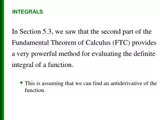
Integrals. 5. Evaluating Definite Integrals. 5.3. Evaluating Definite Integrals. We have computed integrals from the definition as a limit of Riemann sums and we saw that this procedure is sometimes long and difficult.

E N D
Evaluating Definite Integrals • We have computed integrals from the definition as a limit of Riemann sums and we saw that this procedure is sometimes long and difficult. • Sir Isaac Newton discovered a much simpler method for evaluating integrals and a few years later Leibniz made the same discovery. • They realized that they could calculate if they happened to know an antiderivative F of f.
Evaluating Definite Integrals • Their discovery, called the Evaluation Theorem, is part of the Fundamental Theorem of Calculus. • This theorem states that if we know an antiderivative F of f, then we can evaluate simply by subtracting the values of F at the endpoints of the interval [a, b].
Evaluating Definite Integrals • It is very surprising that , which was defined by a • complicated procedure involving all of the values of f(x) for • a x b, can be found by knowing the values of F(x) at only • two points, a and b. • For instance, we know that an antiderivative of the function f(x) = x2 is F(x) = x3, so the Evaluation Theorem tells us that • Although the Evaluation Theorem may be surprising at first glance, it becomes plausible if we interpret it in physical terms.
Evaluating Definite Integrals • If v(t) is the velocity of an object and s(t) is its position at time t, then v(t) = s(t), so s is an antiderivative of v. • We have considered an object that always moves in the positive direction and made the guess that the area under the velocity curve is equal to the distance traveled. In symbols: • That is exactly what the Evaluation Theorem says in this context.
Evaluating Definite Integrals • When applying the Evaluation Theorem we use the notation • and so we can write • where F = f • Other common notations are and .
Example 1 – Using the Evaluation Theorem • Evaluate • Solution: • An antiderivative of f(x) = ex is F(x) = ex, so we use the Evaluation Theorem as follows:
Indefinite Integrals • We need a convenient notation for antiderivatives that makes them easy to work with. • Because of the relation given by the Evaluation Theorem between antiderivatives and integrals, the notation f(x) dx is traditionally used for an antiderivative of f and is called an indefinite integral. Thus
Indefinite Integrals • You should distinguish carefully between definite and indefinite integrals. A definite integral f(x) dx is a number, whereas an indefinite integral f(x) dx is a function (or family of functions). • The connection between them is given by the Evaluation Theorem: If f is continuous on [a, b], then
Indefinite Integrals • If F is an antiderivative of f on an interval I, then the most general antiderivative of f on I is F(x) + C, where C is an arbitrary constant. For instance, the formula • is valid (on any interval that doesn’t contain 0) because (d/dx) ln |x|= 1/x. • So an indefinite integral f(x) dx can represent either a particular antiderivative of f or an entire family of antiderivatives (one for each value of the constant C).
Indefinite Integrals • The effectiveness of the Evaluation Theorem depends on having a supply of antiderivatives of functions. • We therefore restate the Table of Antidifferentiation Formulas, together with a few others, in the notation of indefinite integrals. • Any formula can be verified by differentiating the function on the right side and obtaining the integrand. For instance, • sec2x dx = tan x + C because (tan x + C) = sec2x
Example 3 • Find the general indefinite integral • (10x4 – 2 sec2x) dx • Solution: • Using our convention and Table 1 and properties of integrals, we have • (10x4 – 2 sec2x) dx =10 x4dx – 2 sec2x dx • = 10 – 2 tan x + C • = 2x5 – 2 tan x + C • You should check this answer by differentiating it.
Applications • The Evaluation Theorem says that if f is continuous on [a, b], then • where F is any antiderivative of f. This means that F = f, so the equation can be rewritten as
Applications • We know that F(x) represents the rate of change of y = F(x) with respect to x and F(b) – F(a) is the change in y when x changes from a to b. [Note that y could, for instance, increase, then decrease, then increase again. Although y might change in both directions, F(b) – F(a) represents the net change in y.] • So we can reformulate the Evaluation Theorem in words as follows.
Applications • This principle can be applied to all of the rates of change in the natural and social sciences. Here are a few instances of this idea: • If an object moves along a straight line with position function s(t), then its velocity is v(t) = s(t), so • is the net change of position, or displacement, of the particle during the time period from t1 to t2.
Applications • We have guessed that this was true for the case where the object moves in the positive direction, but now we have proved that it is always true. • If we want to calculate the distance the object travels during the time interval, we have to consider the intervals when v(t) 0 (the particle moves to the right) and also the intervals when v(t) 0 (the particle moves to the left). • In both cases the distance is computed by integrating |v(t)|, the speed. Therefore
Applications • Figure 4 shows how both displacement and distance traveled can be interpreted in terms of areas under a velocity curve. • displacement = • distance = Figure 4
Example 7 – Displacement Versus Distance • A particle moves along a line so that its velocity at time t is v(t) = t2 – t – 6 (measured in meters per second). • (a) Find the displacement of the particle during the time period 1 t 4. • (b) Find the distance traveled during this time period. • Solution: • (a) By Equation 2, the displacement is
Example 7 – Solution cont’d • This means that the particle’s position at time t = 4 is 4.5 m to the left of its position at the start of the time period. • (b) Note that v(t) = t2 – t – 6 = (t – 3)(t + 2) and so v(t) 0 on the interval [1, 3] and v(t) 0 on [3, 4].
Example 7 – Solution cont’d • Thus, from Equation 3, the distance traveled is