Download
1 / 15
160 likes | 350 Views
EE 313 Linear Systems and Signals Fall 2018. Continuous-Time Fourier Transform. Prof. Brian L. Evans Dept. of Electrical and Computer Engineering The University of Texas at Austin. Textbook: McClellan, Schafer & Yoder, Signal Processing First, 2003.

E N D
EE 313 Linear Systems and Signals Fall 2018 Continuous-Time Fourier Transform Prof. Brian L. Evans Dept. of Electrical and Computer Engineering The University of Texas at Austin Textbook: McClellan, Schafer & Yoder, Signal Processing First, 2003 Lecture 15 http://www.ece.utexas.edu/~bevans/courses/signals
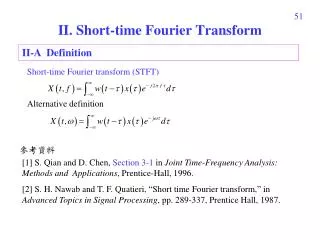
Continuous-Time Fourier Transform – SPFirst Ch. 11 Intro Linear Systems and Signals Topics ✔ ✔ ✔ ✔ ✔ ✔ ✔ ✔ ✔ ✔ ✔ ✔ ✔ ✔ ✔ ✔ ** Spectrograms (Ch. 3) for time-frequency spectrums (plots) computed the discrete-time Fourier series for each window of samples.
Continuous-Time Fourier Transform – SPFirst Ch. 11 Intro Continuous-Time Fourier Transform • General definition of the frequency spectrum Define a precise notion of bandwidth Explain inner workings of communication systems Analyze continuous-time linear time-invariant filters • Periodic signals (SPFirst Ch. 3) Continuous-time periodic signals represented as sum of cosines Cosine frequencies integer multiples of fundamental frequency Fundamental frequency w0 = 2 p / T0;T0 is fundamental period • Linear time-invariant systems (SPFirst Ch. 10) Output frequencies are only those present in input
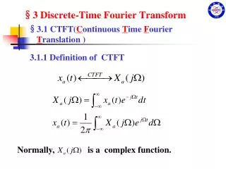
Continuous-Time Fourier Transform – SPFirst Sec. 11-1 Continuous-Time Fourier Transform • Forward direction Analysis: extracts spectrum information from the signal x(t) h(t) d(t) • Inverse direction Synthesis: creates time-domain signal x(t) from its spectral info • Build up transform pairs and properties (pp. 338-339) As we did for z-transforms and we’ll do for Laplace transforms • Example continuous-time Fourier transforms Dirac delta: Delayed Dirac delta: Impulse response of an ideal delay by T seconds
Continuous-Time Fourier Transform – SPFirst Sec. 11-4.1 Causal Exponential Signal w = -8: 0.01 : 8; H = 1 ./ (1 + j*w); Hmag = abs(H); Hphase = phase(H); figure; plot(w, Hmag); title('Magnitude Response'); ylim( [-0.0 1.1] ); figure; plot(w, Hphase); title('PhaseResponse'); • Formula: Magnitude-Phase form Oscillates Decays if Re{a} > 0 a = 1 See lecture slide 14-5 for an example when a = 2
Continuous-Time Fourier Transform – SPFirst Sec. 11-4.2 X(jw) x(t) t F 1 w t -t/2 0 t/2 -6p -4p -2p 2p 4p 6p 0 t t t t t t Rectangular Pulse in Time
From sifting property of Dirac delta, Continuous-Time Fourier Transform – SPFirst Sec. 11-4.4 x(t) = 1 1 t 0 F Impulse in Time or Frequency • Consider Dirac delta in Fourier domain Using linearity property, F{ 1 } = 2pd(w) X(jw) = 2p d(w) (2p) w 0 (2p) indicates area under Dirac delta
Continuous-Time Fourier Transform – SPFirst Sec. 11-4.5 F Two-Sided Cosine Signal X(jw) x(t) = cos(w0t) (p) (p) t w 0 -w0 w0 0
Continuous-Time Fourier Transform – SPFirst Sec. 11-8 t X(jt) F t -6p -4p -2p 2p 4p 6p t t t t t t 0 Duality • Forward/inverse transforms are similar • Example: rect(t / t) tsinc(wt / (2p)) Apply duality tsinc(tt/(2p)) 2 prect(-w/t) rect(·) is even tsinc(tt/(2p)) 2 prect(w/t) 2p w -t/2 0 t/2
Continuous-Time Fourier Transform – SPFirst Sec. 11-5.1 Scaling • For a 0 and given x(t) X(jw) |a| > 1: compress time axis, expand frequency axis |a| < 1: expand time axis, compress frequency axis • Extent in time domain is inversely proportional to extent in frequency domain (a.k.a. bandwidth) x(t) is wider spectrum is narrower x(t) is narrower spectrum is wider
Continuous-Time Fourier Transform – SPFirst Sec. 11-7.1 Shifting in Time • Shifting in time Does not change magnitude of Fourier transform Shifts phase of Fourier transform by –w t0(so –t0 is slope of the linear phase) • Derivation Let u = t – t0, so du = dt and integration limits stay same
Continuous-Time Fourier Transform – SPFirst Sec. 11-8 F F Sinusoidal Amplitude Modulation • Multiplication in time is convolution in frequency • Alternate derivation (SPFirstSec. 12-2.1)
Continuous-Time Fourier Transform – SPFirst Sec. 11-8 X(jw) 1 w -w1 w1 0 Y(jw) 1/2 X(j(w+w0)) 1/2 X(j(w-w0)) 1/2 w -w0 - w1 -w0 + w1 w0 - w1 w0 + w1 0 -w0 w0 Sinusoidal Amplitude Modulation • Example: y(t) = x(t) cos(w0 t) x(t) is ideal lowpass signal with bandwidth w1 < w0 • Demodulation (i.e. recovery of x(t) from y(t)) is modulation followed by lowpass filtering • Similar derivation for modulation with sin(w0 t)
Conditions Continuous-Time Fourier Transform – SPFirst Sec. 11-7.2 Time Differentiation Property f(t) 0 when |t| f(t) is differentiable • Derivation of property:Given f(t) F(jw)
Time Integration Property • Example 15-15