Download
1 / 43
720 likes | 1.6k Views
Continuous-Time Signal Analysis: The Fourier Transform. Chapter 7 Mohamed Bingabr. Chapter Outline. Aperiodic Signal Representation by Fourier Integral Fourier Transform of Useful Functions Properties of Fourier Transform Signal Transmission Through LTIC Systems Ideal and Practical Filters

E N D
Continuous-Time Signal Analysis: The Fourier Transform Chapter 7 Mohamed Bingabr
Chapter Outline • Aperiodic Signal Representation by Fourier Integral • Fourier Transform of Useful Functions • Properties of Fourier Transform • Signal Transmission Through LTIC Systems • Ideal and Practical Filters • Signal Energy • Applications to Communications • Data Truncation: Window Functions
Link between FT and FS Fourier series (FS) allows us to represent periodic signal in term of sinusoidal or exponentials ejnot. Fourier transform (FT) allows us to represent aperiodic (not periodic) signal in term of exponentials ejt. xTo(t)
Link between FT and FS xT(t) xTo(t) As T0 gets larger and larger the fundamental frequency 0 gets smaller and smaller so the spectrum becomes continuous. 0
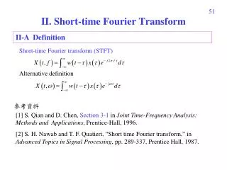
The Fourier Transform Spectrum The Fourier transform: The Amplitude (Magnitude) Spectrum The Phase Spectrum The amplitude spectrum is an even function and the phase is an odd function. The Inverse Fourier transform:
Example Find the Fourier transform of x(t) = e-atu(t), the magnitude, and the spectrum Solution: S-plane s = + j j Re(s) -a How does X() relates to X(s)? ROC Since the j-axis is in the region of convergence then FT exist.
Useful Functions Unit Gate Function 1 x -/2 /2 Unit Triangle Function 1 x -/2 /2
Useful Functions Interpolation Function sinc(x) x
Example Find the FT, the magnitude, and the phase spectrum of x(t) = rect(t/). Answer What is the bandwidth of the above pulse? The spectrum of a pulse extend from 0 to . However, much of the spectrum is concentrated within the first lobe (=0 to 2/)
Find the FT of the unit impulse (t). Answer Find the inverse FT of (). Answer Examples
Find the inverse FT of (- 0). Answer Find the FT of the everlasting sinusoid cos(0t). Answer Examples
Examples Find the FT of a periodic signal. Answer
Examples Find the FT of the unit impulse train Answer
Properties of the Fourier Transform • Linearity: • Let and • then • Time Scaling: • Let • then Compression in the time domain results in expansion in the frequency domain Internet channel A can transmit 100k pulse/sec and channel B can transmit 200k pulse/sec. Which channel does require higher bandwidth?
Left or Right Shift in Time: • Let • then Properties of the Fourier Transform • Time Reversal: • Let • then Example:Find the FT of eatu(-t) and e-a|t| Time shift effects the phase and not the magnitude. Example: if x(t) = sin(t) then what is the FT of x(t-t0)? Example:Find the FT of and draw its magnitude and spectrum
Properties of the Fourier Transform • Multiplication by a Complex Exponential (Freq. Shift Property): • Let • then • Multiplication by a Sinusoid (Amplitude Modulation): • Let • then cos0t is the carrier, x(t) is the modulating signal (message), x(t) cos0t is the modulated signal.
Example: Amplitude Modulation x(t) Example: Find the FT for the signal A -2 2 HW10_Ch7: 7.1-1, 7.1-5, 7.1-6, 7.2-1, 7.2-2, 7.2-4, 7.3-2
Amplitude Modulation Modulation Demodulation Then lowpass filtering
Applic. of Modulation:Frequency-Division Multiplexing 1- Transmission of different signals over different bands 2- Require smaller antenna
Properties of the Fourier Transform • Differentiation in the Frequency Domain: • Let • then • Differentiation in the Time Domain: • Let • then Example: Use the time-differentiation property to find the Fourier Transform of the triangle pulse x(t) = (t/)
Properties of the Fourier Transform • Integration in the Time Domain: • Let • Then • Convolution and Multiplication in the Time Domain: • Let • Then Frequency convolution
Example Find the system response to the input x(t) = e-at u(t) if the system impulse response is h(t) = e-bt u(t).
Properties of the Fourier Transform • Parseval’s Theorem: sincex(t)is non-periodicand has FTX(),then it is an energy signals: Real signal has even spectrum X()= X(-), Example Find the energy of signal x(t) = e-at u(t). Determine the frequency so that the energy contributed by the spectrum components of all frequencies below is 95% of the signal energy EX. Answer: =12.7a rad/sec
Properties of the Fourier Transform • Duality ( Similarity) : • Let • then HW11_Ch7: 7.3-3(a,b), 7.3-6, 7.3-11, 7.4-1, 7.4-2, 7.4-3, 7.6-1, 7.6-6
Data Truncation: Window Functions 1- Truncate x(t) to reduce numerical computation 2- Truncate h(t) to make the system response finite and causal 3- Truncate X() to prevent aliasing in sampling the signal x(t) 4- Truncate Dn to synthesis the signal x(t) from few harmonics. What are the implications of data truncation?
Implications of Data Truncation 1- Spectral spreading 2- Poor frequency resolution 3- Spectral leakage What happened if x(t) has two spectral components of frequencies differing by less than 4/T rad/s (2/T Hz)? The ideal window for truncation is the one that has 1- Smaller mainlobe width 2- Sidelobe with high rolloff rate
Sampling Theorem A real signal whose spectrum is bandlimited to B Hz [X()=0 for || >2B ] can be reconstructed exactly from its samples taken uniformly at a rate fs > 2B samples per second. When fs= 2B then fs is the Nyquist rate.
Example Determine the Nyquist sampling rate for the signal x(t) = 3 + 2 cos(10) + sin(30). Solution The highest frequency is fmax = 30/2 = 15 Hz The Nyquist rate = 2 fmax = 2*15 = 30 sample/sec
Aliasing If a continuous time signal is sampled below the Nyquist rate then some of the high frequencies will appear as low frequencies and the original signal can not be recovered from the samples. Frequency above Fs/2 will appear (aliased) as frequency below Fs/2 LPF With cutoff frequency Fs/2
Quantization & Binary Representation x(t) 111 110 101 100 011 010 001 000 4 3 2 1 0 -1 -2 -3 x L : number of levels n : Number of bits Quantization error = x/2 111 110 101 100 011 010 001 000 4 3 2 1 0 -1 -2 -3
Example A 5 minutes segment of music sampled at 44000 samples per second. The amplitudes of the samples are quantized to 1024 levels. Determine the size of the segment in bits. Solution # of bits per sample = ln(1024) { remember L=2n } n = 10 bits per sample # of bits = 5 * 60 * 44000 * 10 = 13200000 = 13.2 Mbit
Problem 8.3-4 Five telemetry signals, each of bandwidth 1 KHz, are quantized and binary coded, These signals are time-division multiplexed (signal bits interleaved). Choose the number of quantization levels so that the maximum error in the peak signal amplitudes is no greater than 0.2% of the peak signal amplitude. The signal must be sampled at least 20% above the Nyquist rate. Determine the data rate (bits per second) of the multiplexed signal.
Sampling Theorem x(t) x(n) x(t) x(n) t n Link between Continuous and Discrete Continuous Discrete Laplace Transform z Transform x(t) X(s) x(n) X(z) Discrete Fourier Transform Fourier Transform x(t) X(j) x(n) X(k)