Download
1 / 190
1.93k likes | 2k Views
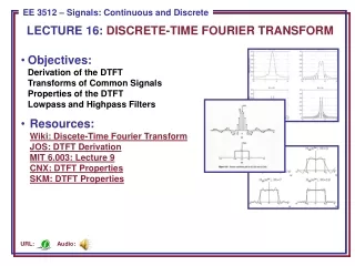
2 Discrete-Time Fourier Transform. Introduce. The signals and systems can be analyzed in time-domain or frequency-domain.

E N D
Introduce • The signals and systems can be analyzed in time-domain or frequency-domain. • In time-domain, any arbitrary sequence can be represented as a weighted linear combination of delayed unit sample sequence, then the input-output relationship of LTI system can be obtained. • The frequency-domain representation of a discrete-time sequence is also discussed in this chapter.
Introduce In many applications, it is convenient to consider an alternate description of a sequence in terms of complex exponential sequences. This leads to a particularly useful representation of discrete-time sequences and certain discrete-time systems in frequency domain.
2.1 The Continuous-Time Fourier Transform We begin with a brief review of the continuous-time Fourier transform, a frequency-domain representation of a continuous-time signal, and its properties, as it will provide a better understanding of the frequency-domain representation of the discrete-time signals and systems, in addition to pointing out the major differences between these two transform.
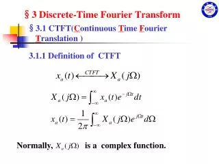
2.1 The Continuous-Time Fourier Transform • Definition of continuous-time FT Continuous-time Fourier transform (CTFT) Inverse continuous-time Fourier transform (ICTFT)
2.1 The Continuous-Time Fourier Transform • Definition of continuous-time FT The CTFT can also be expressed in polar form as where magnitude spectrum phase spectrum
2.1 The Continuous-Time Fourier Transform • Definition of continuous-time FT Dirichlet conditions: (a) The signal has a finite number of finite discontinuous and a finite number of maxima and minima in any finite interval. (b) The signal is absolutely integrable; that is,
2.1 The Continuous-Time Fourier Transform • Energy density spectrum The total energy εx of a finite-energy continuous-time complex signal xa(t) is given by The energy can also be expressed in terms of the CTFT Xa(jΩ) Parseval’s relation
2.1 The Continuous-Time Fourier Transform • Energy density spectrum The energy density spectrum of the continuous-time signal xa(t) is The energy over a specified range of frequencies of the signal can be computed by over this range:
2.1 The Continuous-Time Fourier Transform • Band-limited continuous-time signals a band-limited continuous-time signal has a spectrum that is limited to a portion of the above frequency range. An ideal band-limited signal has a spectrum that is zero outside a finite frequency range However, an ideal band-limited signal cannot be generated in practice.
2.1 The Continuous-Time Fourier Transform • Band-limited continuous-time signals Band-limited signals are classified according to the frequency rang where most of the signal’s energy is concentrated. • lowpass continuous-time signal • highpass continuous-time signal bandpass continuous-time signal
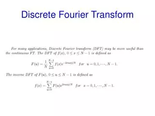
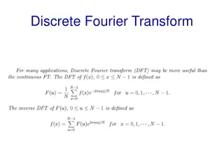
2.2 The Discrete-Time Fourier transform • 2.2.1 Definition of DTFT The discrete-time Fourier transform (DTFT) of a sequence x[n] is defined by As can be seen from the definition, The discrete-time Fourier transform (DTFT) of a sequence x[n] is a function of the normalized angular frequency.
2.2 The Discrete-Time Fourier transform 2.2.1 Definition of DTFT Example 1 Discrete-time Fourier transform of the unit sample sequence
2.2 The Discrete-Time Fourier transform 2.2.1 Definition of DTFT Example 2 Discrete-time Fourier transform of an exponential sequence
2.2 The Discrete-Time Fourier transform • 2.2.1 Definition of DTFT The Fourier coefficients x[n] can be computed from using the Fourier integral given by inverse discrete-time Fourier transform
2.2 The Discrete-Time Fourier transform • 2.2.1 Definition of DTFT For notational convenience, we shall use the operator symbol to denote the DTFT of the sequence x[n]. Likewise, we shall use the operator symbol to denote the inverse Fourier transform. A DTFT pair will denote as
2.2 The Discrete-Time Fourier transform • 2.2.2 Properties of DTFT • Periodicity property Unlike the continuous-time Fourier transform, it is a periodic function in ω with a period 2π . To verify this property, observe that for any integer k,
2.2 The Discrete-Time Fourier transform In general, the Fourier transform is a complex function of the real variable ω and can be written in rectangular form as From above equation, it follows that
2.2 The Discrete-Time Fourier transform The Fourier transform can alternately be expressed in the polar from as where magnitude function phase function
2.2 The Discrete-Time Fourier transform • Example 3 Real and imaginary Parts and Magnitude and phase functions of a discrete-time Fourier transform. Discrete-time Fourier transform of an exponential sequence Where
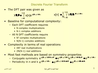
2.2 The Discrete-Time Fourier transform • Symmetry relations We describe here some additional properties of the Fourier transform that are based on the symmetry relations. These properties can simplify the computational complexity and are often useful in digital signal processing applications.
2.2 The Discrete-Time Fourier transform For a given sequence x[n] with a Fourier transform ,it is easy to determine the Fourier transform of its time-reversed sequence x[-n] and the complex conjugate sequence x*[n].
2.2 The Discrete-Time Fourier transform A Fourier transform is defined a conjugate-symmetricfunction of ω if That is,
2.2 The Discrete-Time Fourier transform The Fourier transform is a conjugate-antisymmetric function ofω if That is,
2.2 The Discrete-Time Fourier transform The Fourier transform can been represent as a sum of conjugate-sysmmetric part and conjugate-antisymmetric part where
2.2 The Discrete-Time Fourier transform Likely, the time-domain sequence x[n] can be defined as a conjugate-symmetric and conjugate-antisymmetric sequence of n if
2.2 The Discrete-Time Fourier transform The discrete-time sequence x[n] can been represent as a sum of conjugate-sysmmetric sequence and conjugate-antisymmetric sequence where
2.2 The Discrete-Time Fourier transform A complex-valued Fourier transform x[n], in general, can be expressed as a sum of a real part xre[n] and a imaginary part xim[n]. thus
2.2 The Discrete-Time Fourier transform • Symmetry relations We next derive the Fourier transforms of and , the real and imaginary parts of the sequence x[n], respectively. Then
2.2 The Discrete-Time Fourier transform • Symmetry relations where
2.2 The Discrete-Time Fourier transform • Symmetry relations A complex-valued sequence x[n], in general, can be expressed as a sum of a conjugate-symmetric part xcs[n] and a conjugate-antisymmetric part xca[n] ,thus where
2.2 The Discrete-Time Fourier transform • Symmetry relations We can also derive the Fourier transforms of the conjugate-symmetric and conjugate-antisymmetric parts of a sequence x[n]. We get similarly
2.2 The Discrete-Time Fourier transform • Symmetry relations For a real sequence, thus xim[n]=0 , we have Implying that is a conjugate-symmetric function, thus
2.2 The Discrete-Time Fourier transform • Real and purely sequences Implying that is a conjugate-symmetric function. As a result, the real part and imaginary of the Fourier transform of a real sequence are, respectively, even and odd function ω.
2.2 The Discrete-Time Fourier transform Next, we get Thus, for a signal, it follows from the above that even function of ω odd function of ω
2.2 The Discrete-Time Fourier transform For a real signal, the magnitude function can be easily computing using
2.2 The Discrete-Time Fourier transform For a purely imaginary sequence, , as a result, we have It follows that for a purely imaginary sequence,
2.2 The Discrete-Time Fourier transform • Convergence condition For uniform convergence of
2.2 The Discrete-Time Fourier transform • Convergence condition Absolutely summable (Uniform convergence) Square summable (Mean-square convergence) The Fourier transform may be represented by Dirac delta function
2.2 The Discrete-Time Fourier transform • Discrete-time Fourier transform Theorems • There are a number of important theorems of the discrete-time Fourier transform that are useful in digital signal processing applications. These theorems can be used to determine the Fourier transforms of sequences obtained by combining sequence with known transforms.
2.2 The Discrete-Time Fourier transform • Linearity theorem Let then
2.2 The Discrete-Time Fourier transform • Time-Reversal theorem If Then
2.2 The Discrete-Time Fourier transform • Time-shifting theorem
2.2 The Discrete-Time Fourier transform • Frequency-shifting theorem
2.2 The Discrete-Time Fourier transform • Differentiation-in-frequency theorem
2.2 The Discrete-Time Fourier transform • Convolution theorem
2.2 The Discrete-Time Fourier transform • Modulation theorem
2.2 The Discrete-Time Fourier transform • Parseval’s relation