Download
1 / 46
550 likes | 1.31k Views
Fourier transform. System H ( f ). System h ( t ). Response of Linear Shift-Invariant System. h ( t ). h ( t- ). Input. Output. . t. . t. Output. Input. t. t. Mathematical tool for Signal Analysis of Linear System.

E N D
System H(f) System h(t) Response of Linear Shift-Invariant System h(t) h(t- ) Input Output t t Output Input t t
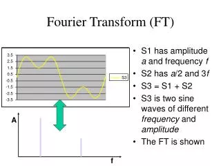
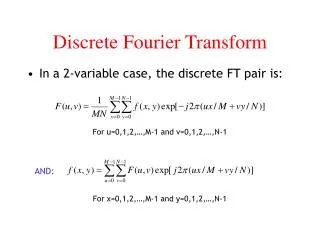
Mathematical tool for Signal Analysis of Linear System • The mathematical tool that relates the frequency-domain description of the signal to its time-domain description is the Fourier transform. • The continuous Fourier transform, or the Fourier transform (FT) for short. • The discrete Fourier transform, or DFT for short.
02_01 Sketch of the interplay between the synthesis and analysis equations embodied in Fourier transformation.
Dirac Delta Function ■Dirac delta function definition G(f) g(t) 1 (t) f t 0
a f (t) (t) f (a) t t ε- ε+ ■Dirac delta function properties
Dirac Comb Function 02_19 g(t) G(f)
g(t) G(f) 1 (f) t f 0 G(f) (f-fc) f 0 fc Example
g(t)=rect(t) t Problem 1 G(f)=sinc(f) f
Problem 2 t G(f)=sinc2(f) f
Problem 3 3. Sinc pulse function
Problem 4 4. Radio frequency (RF) pulse function
Problem 5 t -3 -2 -1 3 2 4 0 1 t -3 -2 -1 3 2 0 1
= t -1 -1 -2 -1 0 1 0 1 Problem 6
f 1 f f f Fourier Transform Table Function g(t) G(f)
f f f f f G(f) Function g(t)
The Inverse Relationship Between Time and Frequency The time-domain and frequency-domain descriptions of a signal are inversely related to each other. A signal cannot be strictly limited in both time and frequency. The bandwidth of a signal provides a measure of the extent of the significant spectral content of the signal for positive frequencies. When the spectrum of a signal is symmetric with a main lobe bounded by well- defined nulls (i.e., frequencies at which the spectrum is zero). A rectangular pulse of duration T seconds has a main spectral lobe of total width (2/T) hertz centered at the origin. The bandwidth of this rectangular pulse is (1/T) hertz. The definition of bandwidth is called the null-to-null bandwidth.
Another popular definition of bandwidth is the 3-db bandwidth. • Yet another measure for the bandwidth of a signal is the root mean-square (rms) bandwidth. • The rms bandwidth of a low-pass signal g(t) with Fourier transform G(f) • Time-Bandwidth Product • (duration) × (bandwidth) = constant • The rms duration of the signal g(t) is
Numerical Computation of the Fourier Transform The fast Fourier transform algorithm is itself derived from the discrete Fourier transform, both time and frequency are represented in discrete form. The discrete Fourier transform provides an approximation to the Fourier transform. If the samples are uniform spaced by Ts seconds, the spectrum of the signal becomes periodic, repeating every fs=1/Ts Hz. Let N denote the number of frequency samples contained in an interval fs. Hence, the frequency resolution involved in the numerical computation of the Fourier transform is defined by where T = NTsis the total duration of the signal.
Interpretations of the DFT and the IDFT • The discrete Fourier transform (DFT) of the sequence gn: Consider then a finite data sequence {g0, g1,…..,,gN-1} which can represent the result of sampling an analog signal g(t) at times t=0, Ts…, (N-1)Ts, where Ts is the sampling interval. The sequence {G0, G1,…GN-1} is called the transform sequence. The inverse discrete Fourier transform (IDFT) of Gk:
Fast Fourier Transform Algorithms FFT algorithms are computationally efficient because they use a greatly reduced number of arithmetic operations as compared to brute force computation of the DFT. An FFT algorithm attains its computational efficiency by following a divide-and-conquer strategy, whereby the original DFT computation is decomposed successively into smaller DFT computations.
The coefficient Wn multiplying yn is called a twiddle factor.
Computation for The Data Sequence 02_35 A signal-flow graph consists of an interconnection of nodes and branches. The direction of signal transmission along a branch is indicated by an arrow. A branch multiplies the variable at a node by the branch transmittance. . 4-point DFT into two 2-point DFTs Trivial case of 2-point DFT 8-point DFT into two 4-point DFTs
The FFT algorithm is referred to as a decimation-in-frequency algorithm, because the transform (frequency) sequence Gk, is divided successively into smaller subsequences. In another popular FFT algorithm, called a decimation-in-time algorithm, the data (time) sequence gn is divided successively into smaller subsequences. P.88
02_02tbl P.88