Download
1 / 24
250 likes | 420 Views
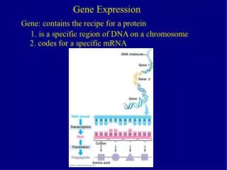
Gene expression profiling identifies molecular subtypes of gliomas. Ruty Shai, Tao Shi, Thomas J Kremen, Steve Horvath, Linda M Liau, Timothy F Cloughesy, Paul S Mischel* and Stanley F Nelson Presented by Stephanie Tsung. Outline. Descriptions of Data Statistical Methods

E N D
Gene expression profiling identifies molecular subtypes of gliomas Ruty Shai, Tao Shi, Thomas J Kremen, Steve Horvath, Linda M Liau, Timothy F Cloughesy, Paul S Mischel* and Stanley F Nelson Presented by Stephanie Tsung
Outline • Descriptions of Data • Statistical Methods • Multidimensional Scaling Plot • Hierarchical Clustering • K-means Clustering • Gene Filtering/Selection • Predictor Comparison • Conclusion/ Future works
Background • Brain tumors can be classified by tumor origins, cell type origin or the tumor site etc; • Tumor classification has been critical in treatment selection and outcome prediction. However, current classification methods are still far from perfect; • As a new technology, DNA microarray has been introduced to cancer classification on the basis of gene expression levels.
Background: Cancer Classification • Cancer classification can be divided into two challenges: class discovery and class prediction. • Class discovery refers to definingpreviously unrecognized tumor subtypes. • Class prediction refersto the assignment of particular tumor samples to already-definedclasses.
Objectives • To test whether gene expression measurements can be used to classify different brain tumors; • To determine sets of significant genes to distinguish brain tumor of different pathological types, grades and survival times; • To validate the selected informative genes in brain tumor classification and prediction.
Data and Pre-Processing • Affymetrix HG-U95Av2 chips • 12,555 Genes and total 42 samples • Tumor Types (#): N(7) O(3) D(18) A(2) AA(3) P(9) • Data pre-processing: • Each tumor was examined by a neuropathologist and dissected into two portions: tissue diagnosis and RNA extraction. • Normalization and Model-Based Expression indices in dChip.
Q. Are the global transcriptional signatures of the different pathologic subtypes of gliomas molecularly distinct?
Multidimensional Scaling Plot (MDS Plot) To uncover the hidden structure of data. D(N) -> D(2) Dimension reduction technique • 12,555 dimensional space to low dimensional Euclidean space • Explain observed similarities and dissimilarity between objects such as correlation, euclidean distance etc. R: cmd1 <- cmdscale(dist(dat1[,1:30]),k=2,eig=T)
MDS Plot Figure 1. (a)Multidimensional scaling plot of all 42 tissue samples plotted in two-dimensional space using expression values from all 12 555 probesets.
Hierarchical Clustering • Evaluate all pair wise distance between objects • Look for a pair with shortest distance • Construct ‘new obj’ by avg. of two obj. • Evaluate distance from ‘new obj’ to all other objects and Go to Step 2 R: h1 <- hclust(dist(x), method=“average”)
III IV Hierarchical Clustering I II Figure 1. (b) The same 42 tissue samples were grouped into hierarchical clusters. Tissue samples are color-coded. I & II : P=0.00006, Fisher’s exact test III & IV : P=0.00001
Ex. 55 8 7 Fisher’s Exact Test Ho: Whether proportion of interest differs between two groups. The two-tailed probability: .326 + .007+ .093 + .163 + .019 = .608
Q. Can we uncover these subtypes without prior knowledge? i.e. How many categories of gliomas are suggested by the gene expression data?
K-means Clustering • To find a K-partition of the observations that minimizes the within sum of squares (WSS) for each clusters • The number of clusters, k, needs to be pre-specified. • Tibshirani prediction strength can be used to determine the optimal k. R: cl1<- kmeans (x, 3)
Figure 2 Grouping of tumors. All tumor samples were plotted using multidimensional scaling using all 12 555 probesets. We performed nonhierarchical Kmeans clustering (Kaufmann and Rousseeu, 1990).
Gene Filtering/Selection • To find the interesting genes which differently expressed in 6 two groups comparisons • Using top 30 genes based on T-test • 170 most differentially expressed genes using T-test
Predictor Comparison • Compare the performance of predictors: Gene Vote • Leave-one-out crossvalidation error rates were calculated. For a given method and sample size, n, a classifier is generated using (n - l) cases and tested on the single remaining case. This is repeated n times, each time designing a classifier by leaving-one-out. Thus, each case in the sample is used as a test case, and each time nearly all the cases are used to design a classifier
Conclusion • Performed MDS plots and K-means clustering analysis and found evidence for three clusters: glioblastomas, lower grade astrocytomas, and oligodendrogilmas (p<0.00001). • A relatively small number of genes can be used to distinguish between molecular subtypes. • Subsets of gliomas can be potentially used for patient stratification and potential targets for treatment.
Future Directions • Construct predictors using different gene selection methods. • Validate the selected genes with new tumor samples. • ……
Number of Cluster (K) 1 2 3 4 5 Tibshirani Prediction Strength 1.000 0.766 0.881 0.501 0.510 K=3 gave us the best prediction power
Statistical problems in response-basedclassification • Identification of new or unknown classes--unsupervised learning • Classification into known classes— supervised learning • Identification of “best” predictor variables—variable selection, e.g. marker genes in microarray data (gene voting, hierarchical clustering)


![[II] Molecular Techniques for Studying Gene Expression](https://cdn2.slideserve.com/4213024/ii-molecular-techniques-for-studying-gene-expression-dt.jpg)