Download
1 / 9
150 likes | 508 Views
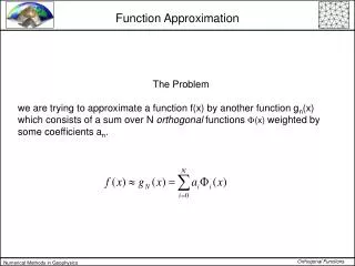
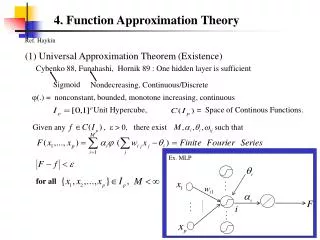
Cybenko 88, Funahashi, Hornik 89 : One hidden layer is sufficient. Sigmoid. Nondecreasing, Continuous/Discrete. Unit Hypercube, = Space of Continous Functions. Given any , > 0, there exist such that. Ex. MLP. for all.

E N D
Cybenko 88, Funahashi, Hornik 89 : One hidden layer is sufficient Sigmoid Nondecreasing, Continuous/Discrete Unit Hypercube, = Space of Continous Functions. Given any , > 0, there exist such that Ex. MLP for all 4. Function Approximation Theory Ref. Haykin (1) Universal Approximation Theorem(Existence) (.) = nonconstant, bounded, monotone increasing, continuous
Barron : Large M for best approximation Small M/N for better empirical fit M may be small if Cf is small. Conflict (2) Mean Squared Error R : ability to generalize / N : # of Training Examples M: # hidden neurons / p : input dimension = regularity or smoothness of f ` , Given mean square error Scalability: The MLP Error is independent of the size of the input space and scales as inverse of the #hidden nodes for large training sets. MLPs are suited to large input Dim. Problems.
(3) Practical Considerations Funahashi : 2 hidden layers are more manageable, In a 1 layer, interaction between neurons makes it difficult to learn. (Hidden= salient feature detector) Sontag : 2 Hidden layers are sufficient to find f -1 from any f ( Inverse problem ) x(n) = f (x(n-1), u(n)) u(n) = f -1(x(n-1), x(n))
u(n) x(n-1) x(n) yi xi Example : Robot Dynamics and Kinematics • Dynamics: x = state u = joint torque • Kinematics: x = Cartesian Position, u = Joint Position (4) Network Jacobian: If the NN has learned the function, then it has learned its Jacobian, too.
Students’ Questions 1. Can the FF net learning take place concurrently (or synchronously) ? 2. Is M = Cf ? 3. Mathematical meaning of the step size, η ? 4. Why do we use the mean square error instead of the first, third order, etc . ? 5. What if more than 2 hidden layers are used ? Any problem then ?
6. BP becomes simple through Jacobian, right ? 7. What do you mean by dividing the input space into local regions ? 8. Where else is Jacobian used, other than in kinematics ? 9. The error can be defined for the global feature by comparing against the desired output. Does each local feature also need a desired output ?
In BackProp, In Network Jacobian Change Error function from EP to Ej Apply BP to xi as weight 1 xi yj NN