Download
1 / 14
150 likes | 183 Views
Filter Approximation Theory. Butterworth, Chebyshev, and Elliptic Filters. Approximation Polynomials. Every physically realizable circuit has a transfer function that is a rational polynomial in s

E N D
Filter Approximation Theory Butterworth, Chebyshev, and Elliptic Filters
Approximation Polynomials • Every physically realizable circuit has a transfer function that is a rational polynomial in s • We want to determine classes of rational polynomials that approximate the “Ideal” low-pass filter response (high-pass band-pass and band-stop filters can be derived from a low pass design) • Four well known approximations are discussed here: • Butterworth: Steven Butterworth,"On the Theory of Filter Amplifiers", Wireless Engineer (also called Experimental Wireless and the Radio Engineer), vol. 7, 1930, pp. 536-541 • Chebyshev: Pafnuty Lvovich Chebyshev (1821-1894) - Russia Cyrillic alphabet -Spelled many ways • Elliptic Function: Wilhelm Cauer (1900-1945) - GermanyU.S. patents 1,958,742 (1934), 1,989,545 (1935), 2,048,426 (1936) • Bessel: Friedrich Wilhelm Bessel, 1784 - 1846 Filter Approximation Theory
|I()|2 1 1 /c Definitions • Let |H()|2 be the approximation to the ideal low-pass filter response |I()|2 Where c is the ideal filter cutoff frequency (it is normalized to one for convenience) Filter Approximation Theory
F() 1 1 Definitions - 2 • |H()|2 can be written as Where F() is the “Characteristic Function” which attempts to approximate: • This cannot be done with a finite order polynomial • provides flexibility for the degree of error in the passband or stopband. Filter Approximation Theory
|H()|2 1 1 Pass band Stop band Transition Region Filter Specification • |H()|2 must stay within the shaded region • Note that this is an incomplete specification. The phase response and transient response are also important and need to be appropriate for the filter application Filter Approximation Theory
|H()|2 1 Butterworth • F() = n and = 1 and • Characteristics • Smooth transfer function (no ripple) • Maximally flat and Linear phase (in the pass-band) • Slow cutoff Filter Approximation Theory
n = 3 Butterworth Continued • Pole locations in the s-plane at:2n = -1 or = (-1)(1/2n) • Poles are equally spaced on the unit circle at =k/2n. • H(s) only uses the n poles in the left half plane for stability. • There are no zeros Filter Approximation Theory
Butterworth Filter |H(s)| for n=4 H(s) = 1/( s4 + 2.6131s3 + 3.4142s2 + 2.6131s + 1) Filter Approximation Theory
Chebyshev – Type 1 • F() = Tn() so T1() = and Tn() = 2 Tn() – Tn-1() • Characteristics • Controlled equiripple in the pass-band • Sharper cutoff than Butterworth • Non-linear phase (Group delay distortion) |H()|2 1 Filter Approximation Theory
Chebyshev |H(s)| for n=4, r=1 (Type 1) Poles lie on an ellipse H(s) = 0.2457/( s4 + 0.9528s3 + 1.4539s2 + 0.7426s + 0.2756) Filter Approximation Theory
|H()|2 1 Elliptic Function • F() = Un() – the Jacobian elliptic function • S-Plane • Poles approximately on an ellipse • Zeros on the j-axis • Characteristics • Separately controlled equiripple in the pass-band and stop-band • Sharper cutoff than Chebyshev (optimal transition band) • Non-linear phase (Group delay distortion) Filter Approximation Theory
Elliptic FunctionH(s) for n=4, rp=3, rs=50 H(s) = (0.0032s4 + 0.0595s2 + 0.1554)/( s4 + 0.5769s3 + 1.2227s2 + 0.4369s + 0.2195) Filter Approximation Theory
Bessel Filter • Butterworth and Chebyshev filters with sharp cutoffs (high order) carry a penalty that is evident from the positions of their poles in the s plane. Bringing the poles closer to the j axis increases their Q, which degrades the filter's transient response. Overshoot or ringing at the response edges can result. • The Bessel filter represents a trade-off in the opposite direction from the Butterworth. The Bessel's poles lie on a locus further from the j axis. Transient response is improved, but at the expense of a less steep cutoff in the stop-band. Filter Approximation Theory
Practical Filter Design • Use a tool to establish a prototype design • MatLab is a great choice • Seehttp://doctord.webhop.net/courses/Topics/Matlab/index.htmfor a Matlab tutorial by Dr. Bouzid Aliane; Chapter 5 is on filter design. • Check your design for ringing/overshoot. • If detrimental, increase the filter order and redesign to exceed the frequency response specifications • Move poles near the j-axis to the left to reduce their Q • Check the resulting filter against your specifications • Moving poles to the left will reduce ringing/overshoot, but degrade the transition region. Filter Approximation Theory