Download
1 / 87
870 likes | 937 Views
Learn about Full and Forward-Only Counterpropagation for function approximation using neural networks. Understand the architecture, algorithms, applications, and examples of these techniques in this comprehensive guide.

E N D
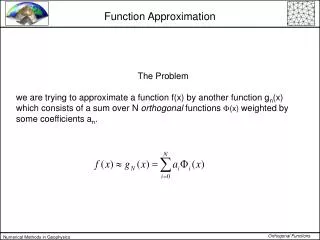
Function Approximation Fariba Sharifian Somaye Kafi
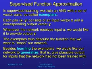
Contents • Introduction to Counterpropagation • Full Counterpropagation • Architecture • Algorithm • Application • example • Forward only Counterpropagation • Architecture • Algorithm • Application • example
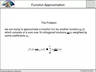
Contents • Function Approximation Using Neural Network • Introduction • Development of Neural Network Weight Equations • Algebra Training Algorithms • Exact Matching of Function Input –Output Data • Approximate Matching of Gradient Data in Algebra Training • Approximate Matching of Function Input-Output Data • Exact Matching of Function Gradient Data
Introduction to Counterpropagation • are multilayer networks based on combination of input, clustering and output layers • can be used to compress data, to approximate functions, or to associate patterns • approximate its training input vectors pair by adoptively constructing a lookup table
Introduction to Counterpropagation (cont.) • training has two stages • Clustering • Output weight updating • There are two types of it • Full • Forward only
Full Counterpropagation • Produces an approximation x*:y* based on • input of an x vector • input of a y vector only • input of an x:y ,possibly with some distorted or missing elements in either or both vectors.
Full Counterpropagation (cont.) • Phase 1 • The units in the cluster layer compete. The learning rule for weight updates on the winning cluster unit is (only the winning unit is allowed to learn)
Full Counterpropagation (cont.) • Phase 2 • The weights from the winning cluster unit J to the output units are adjusted so that the vector of activations of the units in the Y output layer, y*, is an approximation to the input vector y; x*, is an approximation to the input vector x. The weight updates for the units in the Y output and X output layers are
Architecture of Full Counterpropagation X1 w Y1 u Hidden layer Xi Yk Z1 Xn Ym Zj t v Zp Y1* X1* Yk* Xi* Cluster layer Ym* Xn*
Full Counterpropagation Algorithm (phase 1) • Step 1. Initialize weights, learning rates, etc. • Step 2. While stopping condition for Phase 1 is false, do Step 3-8 • Step 3. For each training input pair x:y, do Step 4-6 • Step 4. Set X input layer activations to vector x ; • set Y input layer activations to vector y. • Step 5. Find winning cluster unit; call its index J • Step 6. Update weights for unit ZJ: • Step 7. Reduce learning rate and . • Step 8. Test stopping condition for Phase 1 training
Full Counterpropagation algorithm(phase 2) • Step 9. While stopping condition for Phase 2 is false, do Step 10-16 • (Note: and are small, constant values during phase 2) • Step 10. For each training input pair x:y, do Step 11-14 • Step 11. Set X input layer activations to vector x ; • set Y input layer activations to vector y. • Step 12. Find winning cluster unit; call its index J • Step 13. Update weights for unit ZJ:
Full Counterpropagation Algorithm(phase 2)(cont.) • Step 14. Update weights from unit ZJ to the output layers • Step 15. Reduce learning rate a and b. • Step 16. Test stopping condition for Phase 2 training.
Which cluster is the winner? • dot product (find the cluster with the largest net input) • Euclidean distance (find the cluster with smallest square distance from the input)
Full Counterpropagation Application • The application for counterpropagation is as follows: • Step0: initialize weights. • step1: for each input pair x:y, do step 2-4. • Step2: set X input layer activation to vector x set Y input layer activation to vector Y;
Full Counterpropagation Application (cont.) • Step3: find cluster unit Z, that is closest to the input pair • Step4: compute approximations to x and y: • X*i=tji • Y*k=ujk
Full counterpropagation example • Function approximation of y=1/x • After training phase we have • Cluster unit v w • z1 0.11 9.0 • z2 0.14 7.0 • z3 0.20 5.0 • z4 0.30 3.3 • z5 0.60 1.6 • z6 1.60 0.6 • z7 3.30 0.3 • z8 5.00 0.2 • z9 7.00 0.14 • z10 9.00 0.11
Full counterpropagation example (cont.) X1 Y1 0.11 9.0 Z1 7.0 0.14 5.0 0.2 Z2 . . . 9.0 0.14 0.11 7.0 5.0 Z10 Y1* 0.2 X1*
Full counterpropagation example (cont.) • To approximate value for y for x=0.12 • As we don’t know any thing about y compute D just by means of x • D1=(.12-.11)2 =.0001 D2=.0004 D3=.064 D4=.032 D5=.23 D6=2.2 D7=10.1 D8=23.8 D9=47.3 D10=81
Forward Only Counterpropagation • Is a simplified version of the full counterpropagation • Are intended to approximate y=f(x) function that is not necessarily invertible • It may be used if the mapping from x to y is well defined, but the mapping from y to x is not.
Forward Only Counterpropagation Architecture XY XY w u X1 Y1 Z1 Xi Zj Yk Zp Xn Ym Input layer Cluster layer Output layer
Forward Only Counterpropagation Algorithm • Step 1. Initialize weights, learning rates, etc. • Step 2. While stopping condition for Phase 1 is false, do Step 3-8 • Step 3. For each training input x, do Step 4-6 • Step 4. Set X input layer activations to vector x • Step 5. Find winning cluster unit; call its index j • Step 6. Update weights for unit ZJ: • Step 7. Reduce learning rate • Step 8. Test stopping condition for Phase 1 training.
Step 9. While stopping condition for Phase 2 is false, do Step 10-16 • (Note: is small, constant values during phase 2) • Step 10. For each training input pair x:y, do Step 11-14 • Step 11. Set X input layer activations to vector x ; • set Y input layer activations to vector y. • Step 12. Find winning cluster unit; call its index J • Step 13. Update weights for unit ZJ ( is small) • Step 14. Update weights from unit ZJ to the output layers • Step 15. Reduce learning rate a. • Step 16. Test stopping condition for Phase 2 training.
Forward Only Counterpropagation Application • Step0: initialize weights (by training in previous subsection). • Step1: present input vector x. • Step2: find unit J closest to vector x. • Step3: set activation output units: yk=ujk
Forward only counterpropagation example • Function approximation of y=1/x • After training phase we have • Cluster unit w u • z1 0.5 5.5 • z2 1.5 0.75 • z3 2.5 0.4 • z4 . . • z5 . . • z6 . . • z7 . . • z8 . . • z9 . . • z10 9.5 0.1
Function ApproximationUsing Neural Network Introduction Development of Neural Network Weight Equations Algebra Training Algorithms Exact Matching of Function Input –Output Data Approximate Matching of Gradient Data in Algebra Training Approximate Matching of Function Input-Output Data Exact Matching of Function Gradient Data
Introduction • analytical description for a set of data • referred to as data modeling or system identification
standard tools • Splines • Wavelets • Neural network
Why Using Neural Network • Splines & Wavelets not generalize well to higher 3 dimensional spaces • universal approximators • parallel architecture • trained to map multidimensional nonlinear functions
Why Using Neural Network (cont) • Central to the solution of differential equations. • Provide differentiable closed-analytic- form solutions • have very good generalization properties • widely applicable • translates into a set of nonlinear, transcendental weight equations • cascade structure • nonlinearity of the hidden nodes • linear operations in the input and output layers
Function Approximation Using Neural Network • functions not known analytically • have a set of precise input–output samples • functions modeled using an algebraic approach • design objectives: • exact matching • approximate matching • feedforward neural networks • Data: • Input • Output • And/or gradient information
Objective • exact solutions • sufficient degrees of freedom • retaining good generalization properties • synthesize a large data set by a parsimonious network
Input-to-node values • algebraic training base • if all sigmoidal functions inputs are known weight equations become algebraic • input-to-node values, sigmoidal functions inputs • determine the saturation level of each sigmoid at a given data point
weight equations structure • analyze & train a nonlinear neural network • means • linear algebra • controlling the distribution • controlling the saturation level of the active nodes
Function ApproximationUsing Neural Network Introduction Development of Neural Network Weight Equations Algebra Training Algorithms Exact Matching of Function Input –Output Data Approximate Matching of Gradient Data in Algebra Training Approximate Matching of Function Input-Output Data Exact Matching of Function Gradient Data
Development of Neural Network Weight Equations • Objective • approximate a smooth scalar function of q Inputs • using a feedforward sigmoidal network
Derivative information • can improve network’s generalization properties • partial derivatives with input • can be incorporated in the training set
Network Output • z: computed as a nonlinear transformation • w: input weight • p: input • b: bias • d: output bias • v: output weight • :sigmoid functions • such as: • input-to-node variables
Exactly Match of the Function’s Outputs • output weighted equation
Gradient Equations • derivative of the network output with respect to its inputs
Exact Matching of the Function’s Derivatives • gradient weight equations
Input-to-node Weight Equations • rewriting 12
Four Algebraic Algorithms • Exact Matching of Function Input –Output Data • Approximate Matching of Gradient Data in Algebra Training • Approximate Matching of Function Input-Output Data • Exact Matching of Function Gradient Data
Function ApproximationUsing Neural Network Introduction Development of Neural Network Weight Equations Algebra Training Algorithms Exact Matching of Function Input –Output Data Approximate Matching of Gradient Data in Algebra Training Approximate Matching of Function Input-Output Data Exact Matching of Function Gradient Data
A.Exact Matching of Function Input-Output Data • Input • S is known matrix ps • strategy for producing a well-conditioned S • input weights • o • random number N(0,1) • L scaling factor • user-defined scalar • input-to-node values that do not saturate the sigmoids
Input bias • The input bias d is computed to center each sigmoid at one of the training pairs from
Finally, the linear system in (9) is solved for v by inverting S
Fig. 2-a. Exact input–output-based algebraic algorithm Exact Input-Output-Based Algebraic Algorithm