Supervised Function Approximation
170 likes | 354 Views
Supervised Function Approximation. In supervised learning, we train an ANN with a set of vector pairs, so-called exemplars . Each pair ( x , y ) consists of an input vector x and a corresponding output vector y .

Supervised Function Approximation
E N D
Presentation Transcript
Supervised Function Approximation • In supervised learning, we train an ANN with a set of vector pairs, so-called exemplars. • Each pair (x, y) consists of an input vector x and a corresponding output vector y. • Whenever the network receives input x, we would like it to provide output y. • The exemplars thus describe the function that we want to “teach” our network. • Besides learning the exemplars, we would like our network to generalize, that is, give plausible output for inputs that the network had not been trained with. Neural Networks Lecture 5: The Perceptron
Supervised Function Approximation • There is a tradeoff between a network’s ability to precisely learn the given exemplars and its ability to generalize (i.e., inter- and extrapolate). • This problem is similar to fitting a function to a given set of data points. • Let us assume that you want to find a fitting function f:RR for a set of three data points. • You try to do this with polynomials of degree one (a straight line), two, and nine. Neural Networks Lecture 5: The Perceptron
deg. 2 f(x) deg. 1 deg. 9 x Supervised Function Approximation • Obviously, the polynomial of degree 2 provides the most plausible fit. Neural Networks Lecture 5: The Perceptron
Supervised Function Approximation • The same principle applies to ANNs: • If an ANN has too few neurons, it may not have enough degrees of freedom to precisely approximate the desired function. • If an ANN has too many neurons, it will learn the exemplars perfectly, but its additional degrees of freedom may cause it to show implausible behavior for untrained inputs; it then presents poor ability of generalization. • Unfortunately, there are no known equations that could tell you the optimal size of your network for a given application; there are only heuristics. Neural Networks Lecture 5: The Perceptron
Evaluation of Networks • Basic idea: define error function and measure error for untrained data (testing set) • Typical:where d is the desired output, and o is the actual output. • For classification:E = number of misclassified samples/ total number of samples Neural Networks Lecture 5: The Perceptron
The Perceptron unit i x2 W1 threshold • x1 W2 … f(x1,x2,…,xn) … Wn xn net input signal output Neural Networks Lecture 5: The Perceptron
x0 1 The Perceptron unit i W0 corresponds to - W0 x2 W1 threshold 0 • x1 W2 … f(x1,x2,…,xn) … Wn xn net input signal output Here, only the weight vector is adaptable, but not the threshold Neural Networks Lecture 5: The Perceptron
Perceptron Computation • Similar to a TLU, a perceptron divides its n-dimensional input space by an (n-1)-dimensional hyperplane defined by the equation: • w0 + w1x1 + w2x2 + … + wnxn = 0 • For w0 + w1x1 + w2x2 + … + wnxn > 0, its output is 1, and • for w0 + w1x1 + w2x2 + … + wnxn 0, its output is -1. • With the right weight vector (w0, …, wn)T, a single perceptron can compute any linearly separable function. • We are now going to look at an algorithm that determines such a weight vector for a given function. Neural Networks Lecture 5: The Perceptron
Perceptron Training Algorithm • AlgorithmPerceptron; • Start with a randomly chosen weight vector w0; • Let k = 1; • while there exist input vectors that are misclassified by wk-1, do • Let ij be a misclassified input vector; • Let xk = class(ij)ij, implying that wk-1xk < 0; • Update the weight vector to wk = wk-1 + xk; • Increment k; • end-while; Neural Networks Lecture 5: The Perceptron
Perceptron Training Algorithm • For example, for some input i with class(i) = -1, • If wi > 0, then we have a misclassification. • Then the weight vector needs to be modified to w + w • with (w + w)i < wi to possibly improve classification. • We can choose w = -i, because • (w + w)i = (w - i)i = wi - ii < wi, • and ii is the square of the length of vector i and is thus positive. • If class(i) = 1, things are the same but with opposite signs; we introduce x to unify these two cases. Neural Networks Lecture 5: The Perceptron
Learning Rate and Termination • Terminate when all samples are correctly classified. • If the number of misclassified samples has not changed in a large number of steps, the problem could be the choice of learning rate : • If is too large, classification may just be swinging back and forth and take a long time to reach the solution; • On the other hand, if is too small, changes in classification can be extremely slow. • If changing does not help, the samples may not be linearly separable, and training should terminate. • If it is known that there will be a minimum number of misclassifications, train until that number is reached. Neural Networks Lecture 5: The Perceptron
Guarantee of Success: Novikoff (1963) • Theorem 2.1: Given training samples from two linearly separable classes, the perceptron training algorithm terminates after a finite number of steps, and correctly classifies all elements of the training set, irrespective of the initial random non-zero weight vector w0. • Let wk be the current weight vector. • We need to prove that there is an upper bound on k. Neural Networks Lecture 5: The Perceptron
Guarantee of Success: Novikoff (1963) • Proof: Assume = 1, without loss of generality. • After k steps of the learning algorithm, the current weight vector is • wk = w0 +x1 +x2 +… +xk. (2.1) • Since the two classes are linearly separable, there must be a vector of weights w* that correctly classifies them, that is, sgn(w*ik) = class(ik). • Multiplying each side of eq. 2.1 with w*, we get: • w* wk = w*w0 +w*x1 +w*x2 +… +w*xk. Neural Networks Lecture 5: The Perceptron
Guarantee of Success: Novikoff (1963) • w* wk = w*w0 +w*x1 +w*x2 +… +w*xk. • For each input vector ij, the dot product w*ij has the same sign as class(ij). • Since the corresponding element of the training sequence x = class(ij)ij, we can be assured that • w*x =w*(class(ij)ij) > 0. • Therefore, there exists an > 0 such that w*xi > for every member xi of the training sequence. • Hence: • w* wk > w*w0+ k. (2.2) Neural Networks Lecture 5: The Perceptron
Guarantee of Success: Novikoff (1963) • w* wk > w*w0+ k. (2.2) • By the Cauchy-Schwarz inequality: • |w*wk|2 ||w*||2 ||wk||2. (2.3) • We may assume that that ||w*||= 1, since the unit length vector w*/||w*|| also correctly classifies the same samples. • Using this assumption and eqs. 2.2 and 2.3, we obtain a lower bound for the square of the length of wk: • ||wk||2 > (w*w0+ k) 2. (2.4) Neural Networks Lecture 5: The Perceptron
Guarantee of Success: Novikoff (1963) • Sincewj = wj-1+ xj, the following upper bound can be obtained for this vector’s squared length: • ||wj||2 = wjwj • = wj-1wj-1 + 2wj-1xj + xjxj • = ||wj-1||2 + 2wj-1xj + ||xj||2 • Sincewj-1xj < 0 whenever a weight change is required by the algorithm, we have: • ||wj||2 - ||wj-1||2 < ||xj||2 • Summation of the above inequalities over j = 1, …, k gives an upper bound • ||wk||2 - ||w0||2 < k max ||xj||2 Neural Networks Lecture 5: The Perceptron
Guarantee of Success: Novikoff (1963) • ||wk||2 - ||w0||2 < k max ||xj||2 • Combining this with inequality 2.4: • ||wk||2 > (w*w0+ k) 2 (2.4) • Gives us: • (w*w0+ k) 2 < ||wk||2 < ||w0||2 + k max ||xj||2 • Now the lower bound of ||wk||2 increases at the rate of k2, and its upper bound increases at the rate of k. • Therefore, there must be a finite value of k such that: • (w*w0+ k) 2 > ||w0||2 + k max ||xj||2 • This means that k cannot increase without bound, so that the algorithm must eventually terminate. Neural Networks Lecture 5: The Perceptron