Influence of variations in light and turbulence on ocean carbon dynamics

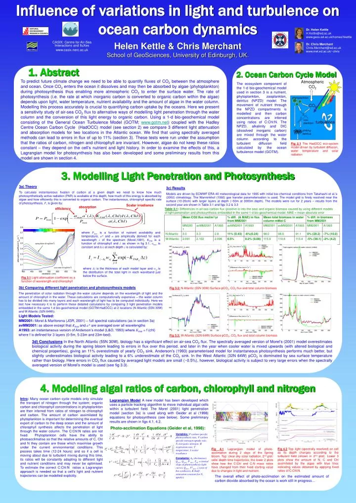
1. Influence of variations in light and turbulence on ocean carbon dynamics turbulence Scalar irradiance absorption efficiency Visible light spectrum green yellow red blue Dr. Helen Kettle H.Kettle@ed.ac.uk www.geos.ed.ac.uk/homes/hkettle Dr. Chris Merchant Chris.Merchant@ed.ac.uk www.met.ed.ac.uk/~chris CASIX: Centre for Air-Sea Interactions and fluXes www.casix.nerc.ac.uk Helen Kettle & Chris Merchant School of GeoSciences, University of Edinburgh, UK. 1. Abstract 2. Ocean Carbon Cycle Model To predict future climate change we need to be able to quantify fluxes of CO2 between the atmosphere and ocean. Once CO2 enters the ocean it dissolves and may then be absorbed by algae (phytoplankton) during photosynthesis thus enabling more atmospheric CO2 to enter the surface water. The rate of photosynthesis (i.e. the rate at which inorganic carbon is converted to organic carbon within the algae) depends upon light, water temperature, nutrient availability and the amount of algae in the water column. Modelling this process accurately is crucial to quantifying carbon uptake by the oceans. Here we present a sensitivity study of air-sea CO2 flux to alternative ways of modelling light penetration through the water column and the conversion of this light energy to organic carbon. Using a 1-d bio-geochemical model consisting of the General Ocean Turbulence Model (GOTM; www.gotm.net) coupled with the Hadley Centre Ocean Carbon Cycle (HadOCC) model (see section 2) we compare 3 different light attenuation and absorption models for two locations in the Atlantic ocean. We find that using spectrally averaged methods can lead to errors in flux of up to 11% (section 3). These tests were run under the assumption that the ratios of carbon, nitrogen and chlorophyll are invariant. However, algae do not keep these ratios constant – they depend on the cell’s nutrient and light history. In order to examine the effects of this, a Lagrangian model for photosynthesis has also been developed and some preliminary results from this model are shown in section 4. Atmospheric CO2 The ecosystem component of the 1-d bio-geochemical model used in section 3 is a nutrient, phytoplankton, zooplankton, detritus (NPZD) model. The movement of nutrient through the NPZD compartments is modelled and then carbon concentrations are inferred using ratios of C:Chl:N. The NPZD, alkalinity and DIC (dissolved inorganic carbon) are mixed through the water column according to the turbulent diffusion field calculated by the ocean turbulence model (GOTM). phytoplankton CO2 zoo-plankton sinking detritus Fig 2.1 The HadOCC eco-system model driven by turbulent diffusion, water temperature and solar radiation 3. Modelling Light Penetration and Photosynthesis 3a) Theory To calculate instantaneous fixation of carbon at a given depth we need to know how much photosynthetically active radiation (PAR) is available at this depth, how much of this energy is absorbed by algae and how efficiently this is converted to organic carbon. The instantaneous, chlorophyll specific rate of photosynthesis, P, is given by: 3c) Results Models are driven by ECMWF ERA-40 meteorological data for 1995 with initial bio-chemical conditions from Takahashi et al.’s (2002) climatology. The Wanninkhof (1992) gas transfer parameterisation is used. The model grid is finely resolved near the surface (10-20cm) with larger layers at depth (~50m at 3000m depth). The models were run for 2 years – results from the second year are shown in Table 3.1 and figs 3.2 & 3.3 Table 3.1: Differences in air-sea carbon flux (positive is into the sea) and organic biomass caused by using different models of light penetration and photosynthesis embedded in the same 1-d bio-geochemical model. MAE = mean absolute error where Pmax is a function of nutrient availability and temperature, a* and a are empirically derived for each wavelength λof the spectrum (Morel,1991), KPAR is a function of chlorophyll and λ as shown in fig 3.1, αmax is constant and I(λ) at each depth z is calculated by: where Δz is the thickness of each model layer and wsj is the distribution of the total light in each waveband just below the surface. Fig 3.1Light attenuation coefficient as a function of wavelength and chlorophyll 3b) Comparing different light penetration and photosynthesis models The penetration of solar radiation through the water column depends on the wavelength of light and the amount of chlorophyll in the water. These calculations are computationally expensive – the water column has to be divided into many layers and each wavelength of light has to be computed individually. Here we test how necessary it is to perform these detailed calculations by comparing 3 light penetration models embedded in the same 1-d bio-geochemical model (GOTM-HadOCC) at 2 locations (N Atlantic (55N 30W) and W Atlantic (32N 64W)). Light Models Tested: MM2001: Morel & Maritorena (JGR, 2001) – full spectral calculations (as in section 3a) avMM2001: as above except that KPAR and a* are averaged over all wavelengths A1993: an instantaneous version of Anderson’s model (L&O, 1993) where KPAR = f (chl) where f is defined for 3 layers (0-5m, 5-23m and 23m-bed). Fig 3.2: N Atlantic (55N 30W) Surface pCO2, CO2 flux and total column biomass Fig 3.3: W Atlantic (32N 64W) Surface pCO2, CO2 flux and total column biomass 3d) Conclusions In the North Atlantic (55N 30W), biology has a significant effect on air-sea CO2 flux. The spectrally averaged version of Morel’s (2001) model overestimates biological activity during the spring bloom leading to errors in flux over this period, and later in the year when cooler water is mixed upwards (with altered biological and chemical properties), giving an 11% overestimate of yearly CO2 sink. Anderson’s (1993) parameterised model for instantaneous photosynthesis performs much better, but slightly underestimates biological activity leading to a 6% underestimate of the CO2 sink. In the West Atlantic (32N 64W) pCO2 is dominated by sea surface temperature rather than biology. Here errors in CO2 flux caused by averaged light models are small (~0.5%), however, biological activity is subject to very large errors when the spectrally averaged version of Morel’s model is used (see fig 3.3). 4. Modelling algal ratios of carbon, chlorophyll and nitrogen Intro: Many ocean carbon cycle models only simulate the transport of nitrogen through the system; organic carbon and chlorophyll concentrations in phytoplankton are then inferred from ratios of nitrogen to chlorophyll and carbon. The amount of carbon assimilated by phytoplankton is important for determining the eventual export of carbon to the deep ocean and the amount of chlorophyll synthesis affects the penetration of light through the water column. The C:Chl:N ratios are not fixed. Phytoplankton cells have the ability to photoacclimatise so that the relative amounts of C, Chl and N they contain are those which maximise growth under the current environmental conditions. This process takes time (12-24 hours) and so if a cell is moving about due to turbulent mixing during this time, its ratios will be constantly adapting to different light and nutrient conditions and may never be optimised. To estimate the correct C:Chl:N ratios a Lagrangian approach is needed so that a cell’s light and nutrient trajectories can be modelled explicitly. Lagrangian Model A new model has been developed which uses a particle tracking algorithm to move individual algal cells within a turbulent field. The Morel (2001) light penetration model (section 3a) is used along with Geider et al (1998) equations for photosynthesis (see below). Some preliminary results are shown in figs 4.1, 4.2. Photo-acclimation Equations (Geider et al, 1998): Variables:P carbon specific photosynthesis rate; V carbon specific nitrogen uptake rate; Ni inorganic nitrogen; R respiration rate; T temperature; I scalar irradiance Constants:AE (Arrhenius), Qmin, Qmax, Pcmax, Tref, α (initial slope of photosynthesis-light curve), Qmax, VCmax, ζ (cost of bio-synthesis), K (half-saturation constant for Ni uptake). Fig 4.2Top: light (spectrally resolved) on cell as its depth changes according to the turbulent field (shown in 2nd plot). Lower 3 plots show the amount of N, C and Chl assimilated by the algae with blue lines indicating values obtained by applying fixed ratios of C:Chl:N. Fig 4.1Lagrangian model of photo-acclimation during 2 days of the Spring bloom. Top: clear sky solar radiation, 2nd plot: cells’ depth-time trajectories; the lower 2 plots show how the C:Chl and C:N mass ratios have changed from their fixed starting value due to changes in light and nutrient. The overall effect of photo-acclimation on the estimated amount of carbon dioxide absorbed by the ocean is work still in progress…