Download
1 / 51
510 likes | 671 Views
Last lecture. Path planning for a moving point Visibility graph Cell decomposition Potential field. Fundamental question of motion planning. Given the geometry of Robot Obstacles Find a path between initial and goal robot positions Key: capture the connectivity of the space.

E N D
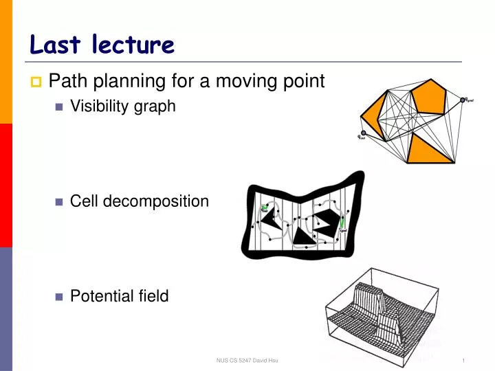
Last lecture • Path planning for a moving point • Visibility graph • Cell decomposition • Potential field NUS CS 5247 David Hsu
Fundamental question of motion planning • Given the geometry of • Robot • Obstacles • Find a path between initial and goal robot positions • Key: capture the connectivity of the space NUS CS 5247 David Hsu
Completeness • A complete motion planner always returns a solution when one exists and indicates that no such solution exists otherwise. • Is the visibility graph algorithm complete? Yes. • How about the exact cell decomposition algorithm and the potential field algorithm? NUS CS 5247 David Hsu
Geometric Preliminaries NUS CS 5247 David Hsu
Primitive objects in the plane class Point { double x; double y; } class Segment { Point p; Point q; } • 0-dim • 1-dim NUS CS 5247 David Hsu
Primitive objects in the plane class Triangle { Point p; Point q; Point r; } • 2-dim class Polygon { list<Point> vertices; int numVertices; } NUS CS 5247 David Hsu
Intersecting primitive objects in the plane ? = • Case 1: line segment & line segment NUS CS 5247 David Hsu
Intersect line segments • Counter-clockwise test c b a isCcw(Point a, Point b, Point c ) { u = b – a; v = c – b; return (u.x*v.y – v.x*u.y) > 0; } NUS CS 5247 David Hsu
Intersect line segments with ccw • Pseudo-code • Special cases isCoincident(Segment s, Segment t) { return xor(isCcw(s.p, s.q, t.p), isCcw(s.p, s.q, t.q)) && xor(isCcw(t.p, t.q, s.p), isCcw(t.p, t.q, s.q)) } NUS CS 5247 David Hsu
Intersecting primitive objects in the plane • Case 2 line segment l & polygon P • Intersect l with every edge of P • Case 3 polygon P & polygon Q • Intersect every edge of P with every edge of Q • More efficient algorithms exist if P or Q are convex. NUS CS 5247 David Hsu
Additional information • Computational geometry • Efficient geometry libraries CGAL, LEDA, etc. NUS CS 5247 David Hsu
Configuration Space NUS CS 5247 David Hsu
How to specify motion? NUS CS 5247 David Hsu
Rough idea • Convert rigid robots, articulated robots, etc. into points • Apply algorithms for moving points NUS CS 5247 David Hsu
Mapping from the workspace to the configuration space workspace configuration space NUS CS 5247 David Hsu
Configuration space • Definitions and examples • Obstacles • Paths • Metrics NUS CS 5247 David Hsu
Configuration space qn q3 q=(q1, q2,…,qn) q1 q2 • The configuration of a moving object is a specification of the position of every point on the object. • Usually a configuration is expressed as a vector of position & orientation parameters: q = (q1, q2,…,qn). • The configuration spaceC is the set of all possible configurations. • A configuration is a point in C. NUS CS 5247 David Hsu
Topology of the configuration pace C = S1x S1 j 2p j f 2p 0 f • The topology of C is usually not that of a Cartesian space Rn. NUS CS 5247 David Hsu
Dimension of configuration space • The dimension of a configuration space is the minimum number of parameters needed to specify the configuration of the object completely. • It is also called the number of degrees of freedom (dofs) of a moving object. NUS CS 5247 David Hsu
Example: rigid robot in 2-D workspace reference direction q y reference point x workspace robot • 3-parameter specification: q = (x, y, q) with q [0, 2p). • 3-D configuration space NUS CS 5247 David Hsu
Example: rigid robot in 2-D workspace x • 4-parameter specification: q = (x, y, u, v) with u2+v2 = 1. Noteu = cosq andv=sinq. • dim of configuration space = ??? • Does the dimension of the configuration space (number of dofs) depend on the parametrization? • Topology: a 3-D cylinder C = R2 x S1 • Does the topology depend on the parametrization? 3 NUS CS 5247 David Hsu
Example: rigid robot in 3-D workspace • q = (position, orientation) = (x, y, z, ???) • Parametrization of orientations by matrix: q = (r11, r12 ,…, r32, r33) where r11, r12 ,…, r33 are the elements of rotation matrixwith • r1i2 + r2i2 + r3i2 = 1 for all i , • r1i r1j + r2i r2j + r3i r3j = 0 for alli ≠ j, • det(R) = +1 NUS CS 5247 David Hsu
Example: rigid robot in 3-D workspace z z z z y f y q y y y x x x x • Parametrization of orientations by Euler angles: (f,q,y) 1 2 34 NUS CS 5247 David Hsu
Example: rigid robot in 3-D workspace • Parametrization of orientations by unit quaternion: u =(u1, u2, u3, u4) with u12+u22 +u32 + u42 = 1. • Note (u1, u2, u3, u4) = (cosq/2, nxsinq/2, nysinq/2, nzsinq/2) with nx2+ny2+nz2 = 1. • Compare with representation of orientation in 2-D:(u1,u2) = (cosq, sinq ) n= (nx, ny, nz) q NUS CS 5247 David Hsu
Example: rigid robot in 3-D workspace • Advantage of unit quaternion representation • Compact • No singularity • Naturally reflect the topology of the space of orientations • Number of dofs = 6 • Topology: R3 x SO(3) NUS CS 5247 David Hsu
Example: articulated robot q2 q1 • q = (q1,q2,…,qn) • Number of dofs = n • What is the topology? An articulated object is a set of rigid bodies connected at the joints. NUS CS 5247 David Hsu
What are the possible representations? What is the number of dofs? What is the topology? Example: protein backbone NUS CS 5247 David Hsu
Configuration space • Definitions and examples • Obstacles • Paths • Metrics NUS CS 5247 David Hsu
Obstacles in the configuration space • A configuration q is collision-free, or free, if a moving object placed at q does not intersect any obstacles in the workspace. • The free spaceF is the set of free configurations. • A configuration space obstacle (C-obstacle) is the set of configurations where the moving object collides with workspace obstacles or with itself. NUS CS 5247 David Hsu
Disc in 2-D workspace workspace configuration space NUS CS 5247 David Hsu
Problem • Input: • Convex polygonal moving object translating in 2-D workspace • Convex polygonal obstacles • Output: configuration space obstacles represented as polygons NUS CS 5247 David Hsu
Observation O • If P is an obstacle in the workspace and M is a moving object. Then the C-space obstacle corresponding to P is P– M. M M P P workspace configuration space NUS CS 5247 David Hsu
Minkowski sum • The Minkowski sum of two sets P and Q, denoted by PQ, is defined asP+Q= { p+q | pP, qQ } • Similarly, the Minkowski difference is defined as P– Q= { p–q | pP, qQ } q p NUS CS 5247 David Hsu
Minkowski sum of convex polygons • The Minkowski sum of two convex polygons P and Q of m and n vertices respectively is a convex polygon P + Q of m + nvertices. • The vertices of P + Q are the “sums” of vertices of P and Q. NUS CS 5247 David Hsu
Computational efficiency • Running time O(n+m) • Space O(n+m) • Non-convex obstacles • Decompose into convex polygons (e.g., triangles or trapezoids), compute the Minkowski sums, and take the union • Complexity of Minkowksi sum O(n2m2) • 3-D workspace NUS CS 5247 David Hsu
Computing C-obstacles robot obstacle NUS CS 5247 David Hsu
Polygonal robot translating in 2-D workspace configuration space workspace NUS CS 5247 David Hsu
Polygonal robot translating & rotating in 2-D workspace configuration space workspace NUS CS 5247 David Hsu
Polygonal robot translating & rotating in 2-D workspace q y x NUS CS 5247 David Hsu
Articulated robot in 2-D workspace workspace configuration space NUS CS 5247 David Hsu
Configuration space • Definitions and examples • Obstacles • Paths • Metrics NUS CS 5247 David Hsu
Paths in the configuration space configuration space workspace • A path in C is a continuous curve connecting two configurations q and q’:such that t(0) = q and t(1)=q’. NUS CS 5247 David Hsu
Constraints on paths • A trajectory is a path parameterized by time: • Constraints • Finite length • Bounded curvature • Smoothness • Minimum length • Minimum time • Minimum energy • … NUS CS 5247 David Hsu
Homotopic paths • Two paths t and t’with the same endpoints are homotopic if one can be continuously deformed into the other:with h(s,0) = t(s) andh(s,1) = t’(s). • A homotopic class of pathscontains all paths that arehomotopic to one another. NUS CS 5247 David Hsu
Example q t2 t1 t3 q’ • t1 and t2 are homotopic • t1 and t3 are not homotopic • Infinity number of of homotopy classes exists. R1 x S1 NUS CS 5247 David Hsu
Connectedness of C-Space • C is connected if every two configurations can be connected by a path. • C is simply-connected if any two paths connecting the same endpoints are homotopic.Examples: R2or R3 • Otherwise C is multiply-connected.Examples: S1 and SO(3) are multiply- connected: • In S1, infinite number of homotopy classes • In SO(3), only two homotopy classes NUS CS 5247 David Hsu
Configuration space • Definitions and examples • Obstacles • Paths • Metrics NUS CS 5247 David Hsu
Metric in configuration space • A metric or distance function d in a configuration space C is a function such that • d(q, q’) = 0 if and only if q = q’, • d(q, q’) = d(q’, q), • . NUS CS 5247 David Hsu
Example q’ • Robot A and a point a on A • a(q): position of a in the workspace when A is at configuration q • A distance d in C is defined byd(q, q’) = maxaA || a(q) -a(q’) ||where ||a - b|| denotes the Euclidean distance between points a and b in the workspace. q NUS CS 5247 David Hsu
Examples in R2 x S1 • Consider R2x S1 • q = (x, y,q),q’ = (x’, y’, q’) with q, q’[0,2p) • a = min { |q - q’| , 2p - |q - q’| } q a q’ ra (x,y) a NUS CS 5247 David Hsu