Download
1 / 68
680 likes | 889 Views
Last lecture. Passive Stereo Spacetime Stereo. Today. Structure from Motion: Given pixel correspondences, how to compute 3D structure and camera motion?. Slides stolen from Prof Yungyu Chuang. Epipolar geometry & fundamental matrix. The epipolar geometry.

E N D
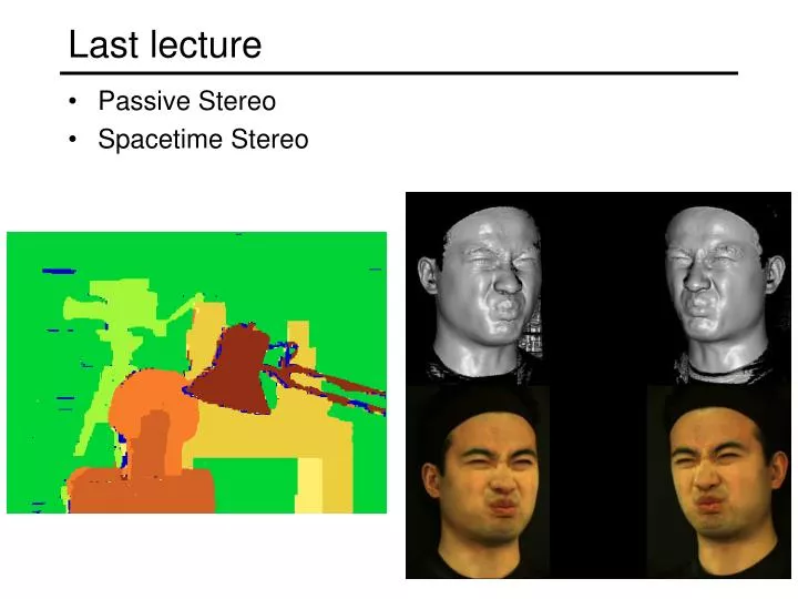
Last lecture • Passive Stereo • Spacetime Stereo
Today • Structure from Motion: Given pixel correspondences, how to compute 3D structure and camera motion? Slides stolen from Prof Yungyu Chuang
The epipolar geometry C,C’,x,x’ and X are coplanar epipolar geometry demo
The epipolar geometry What if only C,C’,x are known?
The epipolar geometry All points on project on l and l’
The epipolar geometry Family of planes and lines l and l’ intersect at e and e’
The epipolar geometry epipolar plane = plane containing baseline epipolar line = intersection of epipolar plane with image epipolar pole = intersection of baseline with image plane = projection of projection center in other image epipolar geometry demo
p p’ T=C’-C Two reference frames are related via the extrinsic parameters The equation of the epipolar plane through X is The fundamental matrix F R C’ C
essential matrix The fundamental matrix F
p p’ T=C’-C The fundamental matrix F R C’ C
Let M and M’ be the intrinsic matrices, then fundamental matrix The fundamental matrix F
p p’ T=C’-C The fundamental matrix F R C’ C
The fundamental matrix F • The fundamental matrix is the algebraic representation of epipolar geometry • The fundamental matrix satisfies the condition that for any pair of corresponding points x↔x’ in the two images
The fundamental matrix F F is the unique 3x3 rank 2 matrix that satisfies x’TFx=0 for all x↔x’ • Transpose: if F is fundamental matrix for (P,P’), then FT is fundamental matrix for (P’,P) • Epipolar lines: l’=Fx & l=FTx’ • Epipoles: on all epipolar lines, thus e’TFx=0, x e’TF=0, similarly Fe=0 • F has 7 d.o.f. , i.e. 3x3-1(homogeneous)-1(rank2) • F is a correlation, projective mapping from a point x to a line l’=Fx (not a proper correlation, i.e. not invertible)
The fundamental matrix F • It can be used for • Simplifies matching • Allows to detect wrong matches
Estimation of F — 8-point algorithm • The fundamental matrix F is defined by for any pair of matches x and x’ in two images. • Let x=(u,v,1)T and x’=(u’,v’,1)T, each match gives a linear equation
8-point algorithm • In reality, instead of solving , we seek f to minimize , least eigenvector of .
8-point algorithm • To enforce that F is of rank 2, F is replaced by F’ that minimizes subject to . • It is achieved by SVD. Let , where • , let • then is the solution.
8-point algorithm % Build the constraint matrix A = [x2(1,:)‘.*x1(1,:)' x2(1,:)'.*x1(2,:)' x2(1,:)' ... x2(2,:)'.*x1(1,:)' x2(2,:)'.*x1(2,:)' x2(2,:)' ... x1(1,:)' x1(2,:)' ones(npts,1) ]; [U,D,V] = svd(A); % Extract fundamental matrix from the column of V % corresponding to the smallest singular value. F = reshape(V(:,9),3,3)'; % Enforce rank2 constraint [U,D,V] = svd(F); F = U*diag([D(1,1) D(2,2) 0])*V';
8-point algorithm • Pros: it is linear, easy to implement and fast • Cons: susceptible to noise
! Problem with 8-point algorithm ~100 ~10000 ~100 ~10000 ~10000 ~100 ~100 1 ~10000 Orders of magnitude difference between column of data matrix least-squares yields poor results
Normalized 8-point algorithm normalized least squares yields good results Transform image to ~[-1,1]x[-1,1] (0,500) (700,500) (-1,1) (1,1) (0,0) (0,0) (700,0) (-1,-1) (1,-1)
Normalized 8-point algorithm • Transform input by , • Call 8-point on to obtain
Normalized 8-point algorithm A = [x2(1,:)‘.*x1(1,:)' x2(1,:)'.*x1(2,:)' x2(1,:)' ... x2(2,:)'.*x1(1,:)' x2(2,:)'.*x1(2,:)' x2(2,:)' ... x1(1,:)' x1(2,:)' ones(npts,1) ]; [U,D,V] = svd(A); F = reshape(V(:,9),3,3)'; [U,D,V] = svd(F); F = U*diag([D(1,1) D(2,2) 0])*V'; [x1, T1] = normalise2dpts(x1); [x2, T2] = normalise2dpts(x2); % Denormalise F = T2'*F*T1;
Normalization function [newpts, T] = normalise2dpts(pts) c = mean(pts(1:2,:)')'; % Centroid newp(1,:) = pts(1,:)-c(1); % Shift origin to centroid. newp(2,:) = pts(2,:)-c(2); meandist = mean(sqrt(newp(1,:).^2 + newp(2,:).^2)); scale = sqrt(2)/meandist; T = [scale 0 -scale*c(1) 0 scale -scale*c(2) 0 0 1 ]; newpts = T*pts;
RANSAC repeat select minimal sample (8 matches) compute solution(s) for F determine inliers until (#inliers,#samples)>95% or too many times compute F based on all inliers
From F to R, T If we know camera parameters Hartley and Zisserman, Multiple View Geometry, 2nd edition, pp 259
Triangulation • Problem: Given some points in correspondence across two or more images (taken from calibrated cameras), {(uj,vj)}, compute the 3D location X CSE 576 (Spring 2005): Computer Vision
Triangulation • Method I: intersect viewing rays in 3D, minimize: • X is the unknown 3D point • Cj is the optical center of camera j • Vj is the viewing ray for pixel (uj,vj) • sj is unknown distance along Vj • Advantage: geometrically intuitive X Vj Cj CSE 576 (Spring 2005): Computer Vision
Triangulation • Method II: solve linear equations in X • advantage: very simple • Method III: non-linear minimization • advantage: most accurate (image plane error) CSE 576 (Spring 2005): Computer Vision
Structure from motion structure for motion: automatic recovery of camera motion and scene structure from two or more images. It is a self calibration technique and called automatic camera tracking or matchmoving. Unknown camera viewpoints
Applications • For computer vision, multiple-view shape reconstruction, novel view synthesis and autonomous vehicle navigation. • For film production, seamless insertion of CGI into live-action backgrounds
Structure from motion geometry fitting 2D feature tracking 3D estimation optimization (bundle adjust) SFM pipeline
Structure from motion • Step 1: Track Features • Detect good features, Shi & Tomasi, SIFT • Find correspondences between frames • Lucas & Kanade-style motion estimation • window-based correlation • SIFT matching
Structure from Motion • Step 2: Estimate Motion and Structure • Simplified projection model, e.g., [Tomasi 92] • 2 or 3 views at a time [Hartley 00]
Structure from Motion • Step 3: Refine estimates • “Bundle adjustment” in photogrammetry • Other iterative methods
Structure from Motion • Step 4: Recover surfaces (image-based triangulation, silhouettes, stereo…) Good mesh
SFM under orthographic projection • Trick • Choose scene origin to be centroid of 3D points • Choose image origins to be centroid of 2D points • Allows us to drop the camera translation: orthographic projection matrix 3D scene point image offset 2D image point
projection of n features in m images W measurement M motion S shape Key Observation: rank(W) <= 3 factorization (Tomasi & Kanade) projection of n features in one image:
solve for known • Factorization Technique • W is at most rank 3 (assuming no noise) • We can use singular value decomposition to factor W: • S’ differs from S by a linear transformation A: • Solve for A by enforcing metric constraints on M Factorization
Trick (not in original Tomasi/Kanade paper, but in followup work) • Constraints are linear in AAT : • Solve for G first by writing equations for every Pi in M • Then G = AAT by SVD Metric constraints • Orthographic Camera • Rows of P are orthonormal: • Enforcing “Metric” Constraints • Compute A such that rows of M have these properties