Download

1 / 41
410 likes | 497 Views
Signal Sampling Requirements. Basic requirements. Some Definitions. Sampling frequency : Rate of extraction of discrete numeric data from an analog continuous signal.

E N D
Signal Sampling Requirements Basic requirements
Some Definitions • Sampling frequency: Rate of extraction of discrete numeric data from an analog continuous signal. • Sampling theorem: The sampling frequency must be higher than twice the highest frequency contained in the signal to allow the original signal to be reconstructed as accurately as desired from the sequence of samples.
Basic Sampling Requirements • Accuracy • Ability of an instrument or method to repeat the observation without deviation. • Precision • Requires the observation to be within some standards. • Resolution defined by Analogue to Digital Converter (ADC).
Digital Resolution • Digital resolution is measured in bits. • Resolution of N bits means that the full range is divided into equal 2N segments. • 8 bit resolution, full range -5 to +5 Volts • 16 bit resolution, full range -5 to +5 Volts
Quantization Error • Let the quantization error probability function be: • Mean value of the error is zero because p(x) is symmetric around 0. • Variance of the error is (in scale units): • Standard deviation:
Example of Quantization Error • Example: 8 bit A/D Converter • Full range of signal is 2^8=256 scale units The peak signal (256∙Δv) to rms noise (0.29 ∙Δv) will be:
Sampling Interval • Assume a continuous signal x(t). • It is sampled at discrete times ti, i=1,n • Sampling interval Δt is the time between two successive sampling times. • Sampling frequency, fs=1/Δt. • Sampling frequency must be fast enough to resolve highest frequency, but oversampling is not practical
Nyquist Frequency • For a given sampling interval Δt the highest frequency that can be resolved is called the Nyquist Frequency (fN): The equation above states that it takes at least 2 sampling intervals to resolve a sinusoidal-type oscillation with period 1/fN.
Sampling Duration, T • Total record length: T=N∙Δt • N: Number of data points • Δt: Sampling interval (=1/fs) Lowest fundamental frequency, fo
Frequency resolution, Δf • Minimum frequency that can be resolved between adjoining components. • In theory we can resolve all frequency components fo to fN with a resolution Δf • Sample long enough (large T) to resolve the low end of the spectrum (fo) and at high resolution (small Δf) • Sample rapidly enough (small Δt) so that you extent the range of frequencies to be resolved (high fN, i.e., high 1/(2Δt))
Raleigh’s Criterion • Two adjacent frequency components are just resolved when the peaks of the spectra are separated by a frequency difference equal or greater than the frequency resolution Δf=1/(N∙Δt). Example from tides: M2 (Lunar Semi-diurnal) has frequency f=0.0805 cph S2 (Solar Semi-diurnal) has frequency f=0.08333 cph Their frequency difference (Δf) is: Δf=0.00282 cph The number of points required to be collected is given by N=1/(Δf·Δt) If sampling (Δt) is every 1 hour, N=71 data points. If sampling (Δt) is every 5 hours, N=355 data points.
Rayleigh Criterion • The Rayleigh Criterion for the separation of two frequencies requires that they should change phase with respect to each other by at least 360o during the record period. • If ω1(=2πf1) and ω2(=2πf2) are the angular frequencies of two signals and T is the record length, the Rayleigh separatioon criterion demands that: • ,
f1=1/10; f2=1/10.2; phi1=0 phi2=pi/3; t=[200:1000]; x1=0.5*cos(2*pi*f1*t+phi1); x2=0.4*cos(2*pi*f2*t+phi2);
Sampling • Sample as long as required to resolve the frequencies required. • Sample as fast as possible to resolve the highest frequencies • Sample accurately enough to reduce noise • Instrument response • No of bits of data per required to raise the value above the noise level (minimum value) • Volume of data to store
Spectral Estimates • If fN is the highest frequency we can measure and fo is the lowest frequency (the limit of frequency resolution) then: • For a time series of N points, we obtain N/2 spectral estimates.
Aliasing Error occurring when the sampling frequency of analog-to-digital conversion is lower than twice the highest frequency contained in the signal (Nyquist frequency). To avoid this error, a low-pass filter should be applied before digitazation
Aliasing Aliasing occurs when the sampling frequency is too low with respect to the frequency content in the original time series. A new, but “false”, frequency is obtained by the sampling procedure.Spectral components above the Nyquist frequency get folded around fNyquist • In general, when a sinusoid of frequency fis sampled with frequencyfs the resulting samples are indistinguishable from those of another sinusoid of frequency fimage(N)=|f-Nfs| for any integer N (withfimage(0)=|f| being the actual signal frequency).Most reconstruction techniques produce the minimum of these frequencies, so it is often important that fimage(0)be the unique minimum.
Aliasing For t=1/2fn All data at frequencies 2 n fn +/- f have the same cosine when sampled at points 1/2fn apart So if you have a Nyquist frequency of fn=100Hz, then energy at f=30Hz can be From 170 (n=1, -f), 230 (n=1,+f), 370 (n=2, -f), 430 (n=2,+f) Hz
Burst vs Continuous Sampling • Collect sample x(k) at time tk: tk=to+k∙Δt • k is an integer • to is the initial time Each sample might have undergone internal averaging or decimation: storing every ith sample average N samples and store the average etc • Burst sampling mode: • Rapid sampling is undertaken over a relative short time interval Δtb • “Burst” is embedded within each regularly spaced time interval Δt
Burst Sampling • ΔtB: Burst length • Δt: Time interval between bursts • n: Number of samples per burst • NB: Number of burst • dt : Sampling interval within each burst Δt ΔtB =n∙dt ΔtB to+n∙dt to to+(NB-1) ∙ Δt+ n∙dt to+(NB-1) ∙ Δt
Different Spectra Spectra from Burst averages Burst Spectra fo=1/T fn=1/2dt fn=1/2Δt fo=1/ΔTB
Stationarity • Stationarity, is defined as a quality of a process in which the statistical parameters (mean and standard deviation) of the process do not change with time. • A weakly stationary process has a constant mean and variance. • A truly stationary process has all higher-order moments constant including the variance and mean.
The most important property of a stationary process is that the auto-correlation function (acf) depends on lag alone and does not change with the time at which the function was calculated. • A weakly stationary process has a constant mean and acf (and therefore variance) • A truly stationary (or strongly stationary) process has all higher-order moments constant including the variance and mean.
Strongly stationary processes are never seen in practice and are discussed only for their mathematical properties. • Weakly stationary processes, are sometimes observed in the real world and are usually assumed to be "close enough" to stationarity in the strict sense (strong stationarity) to be treated as such. • Furthermore, stationarity is really a relative term • Any process that "really" is stationary, can only be seen as stationary if the sampled data from the process is very long compared to the lowest frequency component in the data. In other words, if one collects data for only a short time, short compared to the length of wavelength of the data, then even a stationary process will appear to be nonstationary. • For the purpose of analysis, the stationarity property is a very good thing to have in one’s data, since it leads to many simplifying assumptions. Again, the first step in using any methodology for time series analysis is to check if one’s data is stationary.
Test for Stationarity • Any given sample record will reflect the nonstationary character of the random process in question. • Any given record is too long when compared to the lowest frequency component in the data (excluding a non-stationary mean) • Assume that non-stationary character of the record is revealed by trends in the mean –square-value of the data
Stationarity Test • Divide the sample recorded into N equal time intervals, where the data in each interval can be considered independent. • Compute the mean square value (or mean value and variance independently) for each interval and align these sample values in a time sequence (i.e., <X12>,<X22>,<X32>, …, <XN2>). • Test the sequence above for presence of trends other than those expected due to sampling variations.
Parametric vs Nonparametric Tests • Parametric testing for stationarity (used by people working in the time-domain, i.e., economists; it requires certain assumptions about the nature of the data) • Nonparametric testing for stationarity (used by people working in the frequency domain, i.e., electrical engineers; - black box, we can not make assumptions about the nature of the data) • Nonparametric tests are not based on the knowledge or assumption that the population is normally distributed (Bethea and Rhinehart 1991). By making no assumptions about the nature of the data, nonparametric tests are more widely applicable than parametric tests which often require normality in the data. While more widely applicable, the trade-off is that nonparametric tests are also less powerful than parametric tests. • To arrive at the same statistical conclusion with the same confidence level, nonparametric tests require anywhere from 5% to 35% more data than parametric tests (Bethea and Rhinehart 1991).
The Runs Test (nonparametric) • A run is defined as "a succession of one or more identical symbols, which are followed and preceded by a different symbol or no symbol at all" (Gibbons 1985). • A series of identical flips of a coin is a run, where H represents heads and T for tails, such that: • …THHHHHHTTHTT… • In the example above, the long succession of H is counted as a run of heads. Too few or too many runs is evidence of dependency between the observations, and therefore, nonstationarity. • A runs test is a counting of the number of runs in a series, and comparing the number found to what one would expect if the observations were independent of one another.
Run test for a Time-Series • This test can detect a monotonic trend in a time series x(i), i=1,..., N, by evaluating the number of runs in a second time-series derived from x(i). A "run" is defined as a sequence of identical observations that is followed or preceded by a different observation or no observation at all. • First, the median MD of the observations x(i) is evaluated, and the series y(i) is derived from x(i) as: y(i)=0 if x(i)<MD; y(i)=1 if x(i)>MD or =MD. • Then the number of runs in y(i) is computed. • If x(i) is a stationary random process, the number of runs is a random variable with mean=N/2+1 and variance=(N(N-2))/(4(N-1)). • An observed number of runs significantly different from N/2+1 indicates nonstationarity because of the possible presence of a trend in x(i). A table of runs distribution can be found in (Bendat & Piersol, 1986) – See Table A6
The Runs Test (nonparametric) • Estimate the median value of the whole series, X50 • Find the median value for each one of the N segments, Xi, i=1,N • Subtract the median values Xi-X50 • if Xi-X50>0 assign value 1 • If Xi-X50<0 assign value -1 • Identify runs representing the observations (one run is the group of data with the same sign). Count all runs • HYPOTHESIS: Runs are independent. The acceptance regions for this hypothesis is: [rn;1-a/2 <r <= rn; a/2], with n=N/2 where N = number of observations. • Use Table A.6 (Percentage Points of Run Distribution)) Bendat & Piersol, 1986
Table A.6Percentage Points of Run Distribution Values of rn,a such that Prob [rn>rn;a]=α Where n=N1=N2=N/2 Bendat & Piersol, 1986
Reverse Arrangement Test • The test can detect a monotonic trend in a time series x(i), i=1,..., N. • The method is based on the computation of the number of times that x(i)>x(j) with i<j (each such inequality is called "reversearrangement") for alli. • If the sequence of x(i) are independent observations of the same random variable, then the number of reversearrangement is a random variable with mean=N(N-1)/4 and variance=N(2N+5)(N-1)/72. • An observed number of reverse arrangements significantly different from N(N-1)/4 indicates nonstationarity because of the possible presence of a trend in x(i). Bendat-JS, Persol-AG (1986) Random Data - Analysis and Measurement Procedures, 2nd Edition, John Wiley & Sons, NY
Process The Observations are independent observations of a random variable x where there is no trend. Acceptance region of Hypothesis [AN,1-a/2 < A <= AN,a/2] See Table A.7
Table A.7 Percentage Points of Reverse Arrangement Distribution
Wild Point Editing (Concept) • Calculate the standard deviation of a time-series • Take a moving window of 5 points (Xi,i=1,2,…5) • Sort the data within the window and take the median. • Repeat steps 2 & 3 once more using a 3 point window • Compare original time-series with the twice-sorted one • Find values |Xi-Xi’|>= const*St.dev • Replace value with sorted
Wildpoint.m • function X=wildpoint(Xo,Const) • % • % X=WILD(Xo,[Const]) • % • % Function for wild point editing (spike removal) this technique is recommended only for a small amount of spikes encountered in the signal. is not recommended for noise reduction • % (see Filters) Const is the criterion for spike removal (multiplication factor of STD) • % If omitted Const=2 • % G. Voulgaris (1993) SUDO; Vectorized by GV 2000, USC • % • if nargin==1; Const=2; end • Xstd=std(Xo); • n=length(Xo); • % • Xor=Xo; • % ------- first step --------------------- • I1=[3:(n-2)]'; • il1=size(I1); • xso1=[I1-2*ones(il1) I1-ones(il1) I1 I1+ones(il1) I1+2*ones(il1)]; • xx1=sort(Xo(xso1')); • Xo(I1)=xx1(3,:); • % • % ----------- 2nd step ---------------------- • % • I2=[4:(n-3)]'; • il2=size(I2); • xso2=[I2-ones(il2) I2 I2+ones(il2)+1]; • xx2=sort(Xo(xso2')); • Xo(I2)=xx2(2,:); • % • % Compare original time-series with sorted. • Diferen=abs(Xo-Xor); • III=find(Diferen>Const*Xstd); • X=Xor; • X(III)=Xo(III);
Generate data (x) and then add spikes • dt=0.5; • n=2048; • t=([1:n]-1)*dt; • F=0.07; • x=2.0*cos(2*pi*F*t); • %Add spikes at 3 points • x(500)=x(500)+5; • x(1500)=x(1500)+2; • x(100)=x(100)+1.5;
Use: • Y1=wildpoint(x,1); % remove spikes >1 std • Y2=wildpoint(x,2); % remove spikes >2 std • Y3=wildpoint(x,0.4); % remove spikes >0.4st • The results shown in next page
Corrected data using different criteria 2 largest spikes removed 1 largest spike removed All spikes removed