Download

1 / 42
430 likes | 633 Views
L26: Power Estimation. Battery technology. Microprocessor power dissipation. Power(W). Alpha 21164. Alpha 21264. 50. P III 500. 45. P II 300. 40. 35. Alpha21064 200. 30. 25. P6 166. 20. P5 66. 15. P-PC604 133. 10. i486 DX2 66. P-PC601 50. i486 DX25. 5. i386 DX 16.

E N D
Battery technology Microprocessor power dissipation Power(W) Alpha 21164 Alpha 21264 50 P III 500 45 P II 300 40 35 Alpha21064 200 30 25 P6 166 20 P5 66 15 P-PC604 133 10 i486 DX2 66 P-PC601 50 i486 DX25 5 i386 DX 16 i486 DX4 100 i286 i486 DX 50 P-PC750 400 1980 1985 1990 1995 2000 year Capacity (Watt-Hour/lb) 50 40 Is it possible? 30 20 Nickel-Cadmium 10 1975 1985 1995 2000 1965 year
Cost vs Power Power Strategy Cost Low power processor none none 1 Watt heat sink, air flow $1-5 3-5 Watt Laptop Computer fan sink $10-15 5-15 Watt 15+ Watt exotic $50+
Power Estimation • Circuit Level Power Estimation • Logic/module Level Power Estimation • High Level Power Estimation • Software Power Estimation
Power Estimation Techniques • Circuit Simulation (SPICE): a set of input vectors, accurate, memory and time constraints • Monte Carlo: randomly generated input patterns, normal distributed power per time interval T using a simulator switch level simulation (IRSIM): defined as no. of rising and falling transitions over total number of inputs • Powermill (transistor level): steady-state transitions, hazards and glitches, transient short circuit current and leakage current; measures current density and voltage drop in the power net and identifies reliability problem caused by EM failures, ground bounce and excessive voltage drops. • DesignPower (Synopsys): simulation-based analysis is within 8-15% of SPICE in terms of percentage difference (Probability-based analysis is within 15-20% of SPICE).
Power Estimation Techniques • Static (non-Simulative) - useful for synthesis and architectural exploration • Probability-based • Entropy-based • Dynamic (simulative) - useful for final power • Direct • Sampling-based • Compaction-based • Hybrid (high-level simulation + low-level analytical model evaluation) • Power macromodels for datapath, control, memory • Instruction-level models for microprocessors, DSPs
Previous work(1) • Simulation based approach • accurate and system independent • pattern dependent and after implementation • Direct simulation • SPICE, transistor-level simulator, IRSIM • Statistical simulation • Monte Carlo simulation
Previous work(2) • Non-simulation based approach • library, stochastic, information theoretic model • Behavioral-level approach • library(parameter, area, delay, internal power dissipation) • useful in comparing different adder and multiplier architecture for their switching activity • stochastic • using probability density function, joint probability density function. • Information theoretic • entropy
Previous work(3) • Logic-level approach • using signal probability • zero-delay based approach • OBDD
Circuit Level • SPICE • classical tool for power analysis of circuits • large runtime for large circuits • mainly used as the reference for other power estimation tools. • PowerMill • uses simplified electrical model of the transistor. • operating conditions of transistor are stored as look-up tables.(interpolated by piecewise linear approximation.) • stages - partitioned subcircuits, source/drain connected transistors • 2-3 orders faster than SPICE
Introduction • Glitch • additional power is typically 20%
Circuit Level • IRSIM • event-driven, switch-level simulator • modeled by capacitive nodes and transistors • partitioning into stages is used. • voltage level - High, Low, Undetermined Partitioning into stages
Theoretical background • Synchronous system controlled by global clock
Hierarchical approach to power estimation of combinational circuits(1) • Estimate power of large circuit in a short time • model sub-circuit • compute steady-state prob. • compute edge-activity using state-transition-diagram(std) • compute energy • State-Transition Diagram • 2 input NOR
Hierarchical approach to power estimation of combinational circuits(2)
Hierarchical approach to power estimation of combinational circuits(3) • Computation of steady-state prob. • Compute edge prob. • Make state-transition matrix • Compute steady-state prob. • Compute edge-activity • Energy computation of each edge in the std • Compute edge activity energy using SPICE
Hierarchical approach to power estimation of combinational circuits(4) • Computation of output signal parameters • compute x3 using std of NOR 1 • compute energy for second NOR using Wj calculated NOR 1 and EAj obtained for the second NOR
Hierarchical approach to power estimation of combinational circuits(5) • Loading and routing considerations • Recompute edge energy with concerning of load cap. • Effect of loading can be taken into account
Power estimation of sequential circuits • Sequential block has a combinational block and some storage elements like flip-flop • Extend method to flip-flop
Experimental result(1) • Power estimation of basic cells and multipliers
Logic Level • Pattern dependent analysis • example : Entice-Aspen System(‘94 Workshop on Low Power Design) • cell characterization • using SPICE simulation under different conditions • parameters : supply voltage, input signal slope, operating temperature, fabrication process variation • modeling styles : polynomials, tables, piecewise linear • power vector : Set of logic values and signal transitions • activity analysis • using Verilog-XL simulator • find event vector in the power vector set • total energy = (Energy of power vector)(# of occurrences)
High Level Power Estimation • RTL power estimation • problem • given an RTL circuit description consisting of m modules, and an input vector sequence of length N, estimate the average power consumption • estimation process • perform behavioral simulation and collect the input statistics for all modules in RTL descriptions • evaluate the power macro-model equation for each module and sum over the modules • implementation • in the form of a power co-simulator • collect input statistics from the output of behavioral simulator • produce the power value at the end
Power macro model census macro modeling sampler macro modeling adaptive macro modeling Census macro modeling input data statistics must be collected for every simulation cycle very slow simulation assumed input vectors macro-model is biased ex) pseudo-random, speech data, etc. requires input vectors Power estimate Input vectors Power estimate Behavioral Simulator Sampler Macro Modeling requires input vector power Behavioral Simulator Census Macro Modeling Gate-level Power Simulation input vectors for each module Confidence level and interval Input vectors input vectors for each module vectors confidence level and interval High Level Power Estimation
Sampler macro modeling collects and analyzes input vectors for a relative small number of cycles using statistical random sampling methods Adaptive macro modeling involves a gate-level simulator on a small number of cycles improve the estimation accuracy bias of the static macro models is reduced High Level Power Estimation
High Level Power Estimation • Power estimation at high level • statistical technique • only consider the operations of a given type, number of bus, register and memory access • power dissipation depends on • data activity • physical capacitance • two approaches considering physical cap. • develop analytic models for estimating the switched capacitance • synthesis the circuit and then estimate the power dissipation of the circuit
Develop analytic models develop analytic models for estimation models is a function of the circuit complexity and technology/library parameters key issue estimation of the circuit complexity Synthesis approach procedure quick synthesis estimate power dissipation using RTL/gate-level estimation techniques tends to be more accurate requires the development of a quick synthesis capability much more efficient than a full synthesis program in time High Level Power Estimation
Software Power Estimation • Objective • estimate the power dissipation of a piece of code • Lower level method • gate level power estimation • Higher level method • architectural power estimation • bus switching activity • instruction level power analysis
Gate level power estimation most accurate method too slow approach usefulness evaluate the power dissipation behavior of a processor design characterize the processor for the more efficient instruction Architectural power estimation less precise but much fast determine which system components are active in each execution cycle Bus switching activity bus activity is assumed to be representative of overall switching activity computed from the sequence of op-codes, addresses, and data Instruction level power analysis characterize the power dissipation of instruction sequence use for optimizing a program based on the power estimate Software Power Estimation
Instruction level power analysis base cost independent of the prior state of the processor circuit state effects take into account the effect of prior processor state Instruction Name Base Cost(pJ) Circuit State Effects (pJ) LOAD DLOAD ADD MULT LOAD; ADD LOAD; MULT LOAD 1.98 0.13 0.15 1.19 0.92 1.25 1.06 DLOAD 2.37 0.17 1.19 0.92 1.32 1.06 ADD 0.99 0.26 0.53 0.86 0.99 MULT 1.19 0.66 0.79 0.96 LOAD;ADD 2.10 0.40 0.53 LOAD;MULT 2.25 0.79 Software Power Estimation Circuit State Instruction Base DLOAD A<-x, B<-y 2.37 1.19 LOAD C<-x; MULT D<-A,B 2.25 1.06 0.99 ADD A<-C,D 0.99 Total 5.61 3.24
Power Optimization • Modeling and Technology • Sources of power consumption • Switching component • Short-circuit component • Leakage component • Static power • Voltage Scaling • Adiabatic switching • Circuit Design Level • Logic and Module Design Level • Architecture and System Design Level • Some Design Examples
Switching component • energy for charge parasitic capacitors(gate, diffusion, and interconnect) • ex1. In CMOS, output nodes are charged or discharged. • ex2. Charge sharing PMOS network High NMOS network Low Evaluation
Short circuit component • finite rise and fall time direct current path between Vdd and GND (Both NMOS and PMOS are turned on) Vin Is Is Vin t1 t2
Leakage component • reverse viased PN junction • subthreshold current Gate Gnd P+ P+ N Reverse leakage current Vdd
Static power • although CMOS circuits consume power only when switching, some situations consume static power. • reduced voltage levels feeding CMOS gates • pseudo-NMOS logic style • single PMOS pullup network(always ON because the gate is grounded) • when the output is driven low, conducting path from the supply to ground is created. Vdd-Vtn Vdd Weakly turned on Vdd
Voltage Scaling • Why? • Lowering the supply voltage is most effective means of power reduction. • Feature size of the process geometry decreases. • Smaller process geometry requires the voltage to be lowered because of the thinner gate. • Although the delay increases as the voltage is lowered, the small channel length of the advance process increases the circuit performance
Voltage Scaling • Scaling from 5V to 3.3V • External components(TTL) operate at 5V and the cost to interface with them made the voltage scaling difficult. • The components from low-voltage industry such as LVTTL, CMOS, BiCMOS(which operate at 3.3V) make the voltage scaling with low cost. • Scaling below 3.3V • Depending the technology, the supply voltage can be lower than 3.3V. • The supply voltage cannot be too close to the threshold voltage. significant speed loss.
Performance vs. Voltage scaling • The lowest voltage possible without significant loss of performance is the voltage when the electron velocity get out of saturation. • As the feature size is shrunken, the same electric field can be obtained even when the supply voltage is decreased. ( i.e, velocity saturation occurs at the lower supply voltage. ) electron speed Terminal speed As process technology is shrunken Supply voltage
Adiabatic Switching • Energy injected into a node with cap. C to a voltage, V, is Esig = CV2/2 • Energy drawn from the power supply Einj = QV = CV2 • Einj = 2 Esig : Half of the energy drawn from the supply is dissipated • Also, Esig is dissipated when the node pulled low. • All energy drawn from the supply is used only once before being discarded.
Adiabatic Switching • Solution : charge the load from a supply that is at the same potential as the load • Same supply voltage as the voltage of the load • Charge transfer proceeds sufficiently slowly to not require a large potential drop Energy dissipation varies roughly with the inverse of the switching time • Difficulties • switching transitions must occur when there is no potential drop across the switching devices • zero energy occurs with arbitrarily low speed switching : With realistic switching rates, the energy savings may not sufficient compared to the circuit complexity.
Adiabatic Switching Va X X’ Va Y’ Y • Example : inverter • 1. input(X, X’) set to a value value. • 2. (evaluation) slow voltage ramp to Va from 0 to Vdd. One of Y and Y’ is adiabatically charged to Vdd. • 3. (hold) Y and Y’ can be used as the inputs of other stage • 4. (restore)ramp to Va from Vdd to 0. X Y X’ X X X’ X’ Y’
Adiabatic Switching • Other components of power consumption • on-resistance of switches • Process improvement(parasitic capacitance reduction) allows lower power consumption in adiabatic circuits • Application • When a small number of circuit nodes which significant capacitance driven by high voltage. • Capacitive transcducers, LCD panels, etc.
Reduction of Switched Capacitance • Reduce the switching activity of the digital circuits to the minimal level required to perform the computation saves the power. • Methods • power down mode of the chip • gated clock • circuit optimization to reduce transitions • reduction of # of operations(algorithm change) • data representation • resource ordering • logic style : Dynamic or Static • layout optimization