Download
1 / 19
220 likes | 375 Views
LINEAR PROGRAMMING Introduction to Sensitivity Analysis. Professor Ahmadi. Chapter 3 Linear Programming: Sensitivity Analysis and Interpretation of Solution. Introduction to Sensitivity Analysis Graphical Sensitivity Analysis Spreadsheet Solution & Sensitivity Analysis.

E N D
LINEAR PROGRAMMING Introduction to Sensitivity Analysis Professor Ahmadi
Chapter 3 Linear Programming: Sensitivity Analysis and Interpretation of Solution • Introduction to Sensitivity Analysis • Graphical Sensitivity Analysis • Spreadsheet Solution & Sensitivity Analysis
Sensitivity Analysis • Sensitivity analysis (or post-optimality analysis) is used to determine how the optimal solution is affected by changes, within specified ranges, in: • the objective function coefficients • the right-hand side (RHS) values • Sensitivity analysis is important to the manager who must operate in a dynamic environment with imprecise estimates of the coefficients. • Sensitivity analysis allows the manager to ask certain what-if questions about the problem.
Range of Optimality: The Objective Function Coefficients • A range of optimality of an objective function coefficient is found by determining an interval for the coefficient in which the original optimal solution remains optimal while keeping all other data of the problem constant. (The value of the objective function may change in this range.)
The Right Hand Sides: Shadow Price (Dual Price) • A shadow price for a right hand side value (or resource limit) is the amount the objective function will change per unit increase in the right hand side value of a constraint. • The range of feasibility for a change in the right hand side value is the range of values for this coefficient in which the original shadow price remains constant. • Graphically, a shadow price is determined by adding +1 to the right hand side value in question and then resolving for the optimal solution in terms of the same two binding constraints. • The shadow price is equal to the difference in the values of the objective functions between the new and original problems. • The shadow price for a non-binding constraint is 0.
Example • Refer to the “Woodworking” example of chapter 2, where X1 = Tables and X2= Chairs. The problem is shown below. Max. Z= $100X1+60X2 s.t. 12X1+4X2 < 60 (Assembly time in hours) 4X1+8X2 < 40 (Painting time in hours) The optimum solution was X1=4, X2=3, and Z=$580. Answer the following questions regarding this problem.
Answer the following Questions: 1. Compute therange of optimalityfor the contribution of X1 (Tables) 2. Compute therange of optimalityfor the contribution of X2 (Chairs) 3. Determine thedual Price (Shadow Price) for the assembly stage. • Determine thedual Price (Shadow Price) for the painting stage.
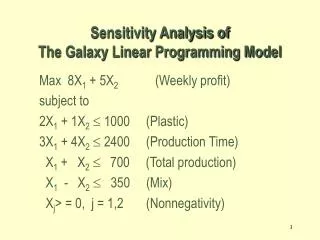
Example 2: Your Turn • Refer to The Olympic Bike Co. (From Chapter 2) • Solve this Problem and find the optimum solution. Max 10x1 + 15x2 (Total Weekly Profit) s.t. 2x1 + 4x2 < 100 (Aluminum Available) 3x1 + 2x2 < 80 (Steel Available) x1, x2 > 0 (Non-negativity)
Example 2: Olympic Bike Co. • Range of Optimality Question: Suppose the profit on deluxe frames is increased to $20. Is the above solution still optimal? What is the value of the objective function when this unit profit is increased to $20? Answer:
Example 2: Olympic Bike Co. • Range of Optimality Question: If the unit profit on deluxe frames were $6 instead of $10 would the optimal solution change? Answer:
Range of Feasibility • The range of feasibility for a change in a right-hand side value is the range of values for this parameter in which the original shadow price remains constant.
Example 2: Olympic Bike Co. • Range of Feasibility and Relevant Costs Question: If aluminum were a relevant cost, what is the maximum amount the company should pay for 50 extra pounds of aluminum? Answer:
Example 3 • Consider the following Minimization linear program: Min Z = 6x1 + 9x2 ($ cost) s.t. x1 + 2x2 < 8 10x1 + 7.5x2 > 30 x2 > 2 x1, x2> 0 Use Excel to solve this problem.
Example 3 • Optimal Solution According to the output: x1 = 1.5 x2 = 2.0 Z (the objective function value) = 27.00.
Example 3 • Range of Optimality Question: Suppose the unit cost of x1 is decreased to $4. Is the current solution still optimal? What is the value of the objective function when this unit cost is decreased to $4? Answer:
Example 3 • Range of Optimality Question: How much can the unit cost of x2 be decreased without concern for the optimal solution changing? Answer:
Example 3 • Range of Feasibility Question: If the right-hand side of constraint 3 is increased by 1, what will be the effect on the optimal solution? Answer:
A Note on Sunk Cost and Relevant Cost • A resource cost is a relevant cost if the amount paid for it is dependent upon the amount of the resource used by the decision variables. • Relevant costs are reflected in the objective function coefficients. • A resource cost is a sunk cost if it must be paid regardless of the amount of the resource actually used by the decision variables. • Sunk resource costs are not reflected in the objective function coefficients.
Reduced Cost • The reduced cost for a decision variable whose value is 0 in the optimal solution is the amount the variable's objective function coefficient would have to improve (increase for maximization problems, decrease for minimization problems) before this variable could assume a positive value. • The reduced cost for a decision variable with a positive value is 0.