Download
1 / 24
240 likes | 342 Views
Comparison of L3 CCI Ozone, Aerosols, and GHG data with models outputs using the CMF. Rossana Dragani ECMWF rossana.dragani@ecmwf.int. The Climate Monitoring Facility (CMF).

E N D
Comparison of L3 CCI Ozone, Aerosols, and GHG data with models outputs using the CMF Rossana Dragani ECMWF rossana.dragani@ecmwf.int
The Climate Monitoring Facility (CMF) • An interactive interface to visualize and facilitate model-observation confrontation for L3 products with a focus on multi-year variability of statistical averages (monthly/regional means). • The CMF Database includes pre-calculated statistical averages of 100+ distinct variables defined over 32 different geographical regions, 12-18 layers (if applicable), several data streams (various reanalyses and several CCI datasets). • Uncertainties compared with either the spread of an Ensemble of DA runs (if available) – infers the climate variability - or observation residuals from their model equivalent. • CMF usage and disclaimer: • It should be used for the applications it was designed for: • Monitoring – as opposed to assessing –data, i.e. spotting potential issues that need to be investigated further; • Looking at long-term variability, multi-year homogeneity (jumps, unrealistic changes,…) and consistency with related variables. • To bear in mind: • Differences in data sampling: Models are defined ‘everywhere’, observations are not; • Refinements (e.g. AK convolution) are not considered.
L3 Ozone data availability *ERS-2 GOME ozone profiles (RAL, and precursor of CCI NPO3 for 1997) were assimilated from Jan 1996-Dec 2002 the comparisons in 1997 are not independent.
(Merged) Tropical total column O3 • CCI Sdev • JRA-25 • Generally good agreement between CCI TCO3 and the European reanalyses. • Agreement with ERA-Interim degrades when reanalyses only constrained by total columns • JRA-25 shows much lower TCO3 than the other datasets. Estimated uncertainty (DU) • The observation uncertainty is comparable with its residuals from the two European reanalyses and the ensemble spread. Ensemble spread Obs - ERA-Int Obs - MACC Observation uncertainty (DU)
Nadir Profile Ozone (NPO3) 5 5 hPa 10 10 hPa CCI NPO3 ERA-Interim MACC 100 x (Obs – ERA-Int) / ERA-Int (%) 30 30 hPa SAGEHALOE 1997 100 hPa
Nadir Profile Ozone (NPO3) 5 hPa 10 hPa CCI NPO3 SDEV Ensemble Spread 30 hPa 100 hPa
(Merged) Limb Profile Ozone (LPO3) CCI LPO3 ERA-Interim MACC 2007 2008 CCI LPO3 SDEV Ensemble Spread
CCI AOD vs. MACC AOD (Oceans, 2008) ADV1.42 SU4.0 ADV1.42 SU4.1 SU4.2 659nm 550nm ORAC2.02 MACC 1610nm 865nm • Agreement typically within the obs error bars.
CCI AOD vs. MACC AOD (550 nm, Oceans, 2008) SU 4.0 SU 4.1 SU 4.2 Global ORAC2.02 ADV1.42 MACC @550nm • Assimilation could improve future AOD reanalysis • Preliminary results based on one month of ADV AATSR assimilation by MACC team show • good synergy with MODIS; • the AATSR+MODIS AOD analyses have the best fit to AERONET data compared to the analyses constrained with either MODIS or AATSR.
Long-term behaviour (SU4.1 & ADV 1.42) SU4.1 ADV1.42 AOD550 AOD659 AOD865 AOD1610
AOD (550nm) over land and oceans Global MACC SU4.1 ADV1.42 Land Oceans
Data availability & usage MCO2 and MCH4 are Fc runs with optimized fluxes from the flux inversion • The CO2 fluxes were optimized using only surface observations (no satellite data included). • The CH4 fluxes were obtained using both SCIAMACHY and surface observations.
CO2 long-term behaviour BESD OCFP SRFP Mean anomaly (ppm) BESD
CCI CO2 vs. MACC CO2 • Good agreement at midlatitudes in the NH • In the tropics and midlatitudes in the SH: • Good agreement between SCIA BESD and GOSAT OCFP, while GOSAT SRFP seems lagged in time. • MCO2 shows a slower CO2 growth with time than in the retrievals. Possible issues: • The CO2 fluxes optimized using only surface observations which are more sparse in the tropics and SH. • Difference in the transport models used in the flux inversion and in the forward calculations likely to be also larger in data sparse regions 20-60N BESD OCFP SRFP MCO2 20S-20N 20-60S
CH4 long-term behaviour IMAP SRFP WFMD OCPR Global • There seems to be some differences in the trends and mean evolution between the products (even for the same instrument): • Differences are small, possibly not statistically significant when normalized to mean CH4; • Some areas might be too small to be significant; • Yet, the two algorithms give different outcome is there scope for a “merged” algorithm with the best features of the two currently available?
CCI CH4 vs. MACC CH4 • Good level of agreement between the four CCI products, particularly in the extra-tropics. • MACC is ~ 100ppb low biased compared with the GHG_CCI, while MCH4 shows a very high level of agreement with the corresponding retrievals. • A sudden change is noticeable in the IMAP SCIAMACHY product (grey lines) at the beginning of 2010 in the tropics and in the NH extra-tropics. • Uncertainties: • The SCIA retrievals have much larger uncertainties than the residuals between the CH4 observations and their MCH4 model equivalent. • In some cases the IMAP retrievals have larger than usual uncertainties. • Increased values in the WFMD product in 2005 following instrumental problems.
Conclusions • Ozone: • TCO3: agreement with ERA-Int higher when the latter constrained by vertically resolved O3 data • Profiles: Retrievals show lower values than the reanalyses. In the region of the O3 maximum (10hPa), the differences from ERA-Int seem consistent with the reanalysis validation. Further investigation of the region below the O3 maximum (30hPa) is needed for NPO3; • L3 uncertainties generally well comparable with O-A residuals and Ensemble Spread. • Aerosols: • Residuals from MACC are within the observation errors. The differences can largely be explained by the +ve bias in the MODIS data (especially in summer). • SU 4.0-4.2: Residuals from MACC increased in the latest versions, but they are consistent with MACC-Aeronet comparisons and likely due to shortcomings in the sea-salt model. • SU4.1 and ADV1.42 retrievals globally show good long-term stability land/ocean differences. • GHG: • Generally good agreement between retrievals and the MACC Fc runs with optimized fluxes • CO2 shows about 2ppm mean growth rate (consistent with e.g. NOAA ESRL data). • In the tropics, the SRFP GOSAT product appears lagged compared with the other datasets. • The SCIA CH4 datasets show small differences in the long-term variability between algorithms. • A sudden change was seen in the IMAP SCIA product in 2010 (in the tropics and northern midlatitudes).
XCO2 20-60N • Good agreement at midlatitudes in the NH • In the tropics and midlatitudes in the SH: • Good agreement between SCIA BESD and GOSAT OCFP, while GOSAT SRFP seems lagged in time. • MCO2 shows a slower CO2 growth with time than in the retrievals. Possible issues: • The CO2 fluxes optimized using only surface observations which are more sparse in the tropics and SH. • Difference in the transport models used in the flux inversion and in the forward calculations likely to be also larger in data sparse regions • Sudden increase in MCO2 end of 2004 and beginning of 2005 significant drought in the Amazonian and Central African regions. BESD OCFP SRFP BESD OCFP SRFP MCO2 20S-20N 20-60S
How can we assess uncertainties with the CMF? • An approach consists in generating an ensemble of DA runs: • Members initialised from slightly different, but equally probable initial conditions. • The ensemble spread (ES) used as proxy of the internal climate variability of a given variable (e.g. Houtekamer and Mitchell, 2001; Evensen, 2003) • It can be used to estimate the uncertainties when not available or when available to assess their quality. • Model bias and any other model issues should have similar effects on all members of the ensemble • As part of the ERA-CLIM project, ECMWF has run an ensemble of low resolution 4D-Var data assimilation runs from the beginning of the 20th century onwards. • ES from these simulation is used to assess the “area typical” CCI O3 uncertainties: a: Geographical area t: time i: ith grid point Na: Points in area a