Download
1 / 1
10 likes | 157 Views
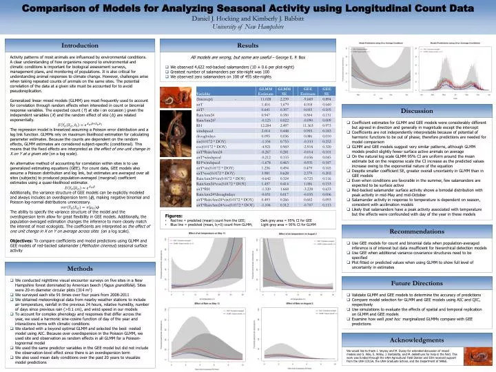
Comparison of Models for Analyzing Seasonal Activity using Longitudinal Count Data Daniel J. Hocking and Kimberly J. Babbitt University of New Hampshire. Introduction. Results.

E N D
Comparison of Models for Analyzing Seasonal Activity using Longitudinal Count Data Daniel J. Hocking and Kimberly J. Babbitt University of New Hampshire Introduction Results Activity patterns of most animals are influenced by environmental conditions. A clear understanding of how organisms respond to environmental and climatic conditions is important for biological assessment surveys, management plans, and monitoring of populations. It is also critical for understanding animal responses to climate change. However, challenges arise when taking repeated counts of animals on the same sites. The potential correlation of the data at a given site must be accounted for to avoid pseudoreplication. Generalized linear mixed models (GLMM) are most frequently used to account for correlation through random effects when interested in count or binomial response variables. The expected count (Y) at site i on occasion j given the independent variables (X) and the random effect of site (bi) are related exponentially. The regression model is linearized assuming a Poisson error distribution and a log link function. GLMMs rely on maximum likelihood estimation for calculating parameter estimates. Because the counts are dependent on the random effects, GLMM estimates are considered subject-specific (conditional). This means that the fixed effects are interpreted as the effect of one unit change in X on Y at a given site (on a log scale). An alternative method of accounting for correlation within sites is to use generalized estimating equations (GEE). For count data, GEE models also assume a Poisson distribution and log link, but estimates are averaged over all sites (subjects) to produced population-averaged (marginal) coefficient estimates using a quasi-likelihood estimator. Additionally, the variance structure of GEE models can be explicitly modeled and always includes an overdispersion term (ϕ), making negative binomial and Poisson log-normal distributions unnecessary. The ability to specify the variance structure of the model and the overdispersion term allow for great flexibility in GEE models. Additionally, the population-averaged estimation changes the inference to more closely match the interest of most ecologists. The coefficients are interpreted as the effect of one unit change in X on Y on average across sites (on a log scale). Objectives: To compare coefficients and model predictions using GLMM and GEE models of red-backed salamander (Plethodoncinereus) seasonal surface activity • All models are wrong, but some are useful – George E. P. Box • We observed 4,622 red-backed salamanders (10 ± 0.6 per plot-night) • Greatest number of salamanders per site-night was 100 • We observed zero salamanders on 100 of 455 site-nights Discussion • Coefficient estimates for GLMM and GEE models were considerably different but agreed in direction and generally in magnitude except the intercept • Coefficients are not independently interpretable because of potential of harmonic functions to be out of phase; therefore predictions are needed for model comparison • GLMM and GEE models suggest very similar patterns, although GLMM models predict slightly fewer surface active animals on average • On the natural log scale GLMM 95% CI are uniform around the mean estimate but on the response scale the CI increase as the predicted values increase owing to the exponential nature of the equation • Despite smaller coefficient SE, greater overall uncertainty in GLMM than in GEE models • Even when conditions are favorable in the summer, few salamanders are expected to be surface active • Red-backed salamander surface activity shows a bimodal distribution with peak activity in mid-May and mid-October • Salamander activity in response to temperature is dependent on season, consistent with acclimation models • Likely that salamanders have a peak activity associated with temperature but the effects were confounded with day of the year in these models • Figures: • Red line = predicted (mean) count from the GEE; Dark grey area = 95% CI for GEE • Blue line = predicted (mean, bi=0) count from GLMM; Light grey area = 95% CI for GLMM Recommendations • Use GEE models for count and binomial data when population-averaged inference is of interest but data insufficient for hierarchical detection models • Use GEE when additional variance-covariance structures need to be specified • Plot fitted or predicted values when using GLMM to show full level of uncertainty in estimates Methods • We conducted nighttime visual encounter surveys on five sites in a New Hampshire forest dominated by American beech (Fagusgrandifolia). Sites were 20-m diameter circular plots (314 m2) • We surveyed each site 91 times over four years from 2008-2011 • We obtained meteorological data from nearby weather stations to include air temperature, rainfall in the previous 24 hours, relative humidity, number of days since previous rain (>0.1 cm), and wind speed in our models • To account for complex phenology and responses that differ across the year, we used a harmonic sine-cosine function of day of the year and interactions terms with climatic conditions • We started with a beyond optimal GLMM and selected the best nested model using AIC. Because over overdispersion in the Poisson GLMM, we used site and observation as random effects in all GLMM for a Poisson-lognormal model • We used the same predictor variables in the GEE model but did not include the observation-level effect since there is an overdispersion term • We also used mean daily conditions over the past 20 years to visualize model predictions Future Directions • Validate GLMM and GEE models to determine the accuracy of predictions • Compare model selection for GLMM and GEE models using AIC and QIC, respectively • Use simulations to evaluate the effects of spatial and temporal replication on GLMM and GEE models • Examine how well post hoc marginalized GLMMs compare with GEE predictions Acknowledgments We would like to thank J. Veyseyand M. Ducey for extended discussion of mixed models and S. Wile, E. Willey, J. Bartolotta, and M. deBethune for help in the field. This work was funded through the UNH Agricultural Field Station and DJH received support from the UNH COLSA, the UNH Graduate School, and the Department of NR&E.