Download

1 / 48
480 likes | 593 Views
Seeking Interpretable Models for High Dimensional Data. Bin Yu Statistics Department, EECS Department University of California, Berkeley http://www.stat.berkeley.edu/~binyu. Basically, I am not interested in doing research and I never have been. I am interested in understanding,

E N D
Seeking Interpretable Models for High Dimensional Data Bin Yu Statistics Department, EECS Department University of California, Berkeley http://www.stat.berkeley.edu/~binyu
Basically, I am not interested in doing research and I never have been. I am interested in understanding, which is quite a different thing. David Blackwell (1919-- )
Characteristics of Modern Data Problems • Goal: efficient use of data for: • Prediction • Interpretation (proxy: sparsity) • Larger number of variables: • Number of variables (p) in data sets is large • Sample sizes (n) have not increased at same pace • Scientific opportunities: • New findings in different scientific fields • Insightful analytical discoveries
Today’s Talk • Understanding early visual cortex area V1 through fMRI • Occam’s Razor • M-estimation with decomposable regularization: L2-error bounds via a unified approach • Learning about V1 through sparse models (pre-selection via corr, sparse linear, sparse nonlinear) • Future work
Understanding visual pathway Gallant Lab at UCB is a leading vision lab. Da Vinci (1452-1519) Mapping of different visual cortex areas PPoPolyak (1957) Small left middle grey area: V1
Understanding visual pathway through fMRI One goal at Gallant Lab: understand how natural images relate to fMRI signals
Gallant Lab in Nature News This article is part of Nature's premium content. Published online 5 March 2008 | Nature | doi:10.1038/news.2008.650 Mind-reading with a brain scan Brain activity can be decoded using magnetic resonance imaging. Kerri Smith Scientists have developed a way of ‘decoding’ someone’s brain activity to determine what they are looking at. “The problem is analogous to the classic ‘pick a card, any card’ magic trick,” says Jack Gallant, a neuroscientist at the University of California in Berkeley, who led the study.
Stimuli Natural image stimuli
Stimulus to fMRI response Natural image stimuli drawn randomly from a database of 11,499 images Experiment designed so that response from different presentations are nearly independent fMRI response is pre-processed and roughly Gaussian
“Neural” (fMRI) encoding for visual cortex V1 Predictor : p=10,921 features of an image Response: (preprocessed) fMRI signal at a voxel n=1750 samples Goal: understanding human visual system interpretable (sparse) model desired good prediction is necessary Minimization of an empirical loss (e.g. L2) leads to • ill-posed computational problem, and • bad prediction
Linear Encoding Model by Gallant Lab Data • X: p=10921 dimensions (features) • Y: fMRI signal • n = 1750 training samples Separate linear model for each voxel via e-L2boosting (or Lasso) Fitted model tested on 120 validation samples • Performance measured by predicted squared correlation
Modeling “history” at Gallant Lab • Prediction on validation set is the benchmark • Methods tried: neural nets, SVMs, e-L2boosting (Lasso) • Among models with similar predictions, simpler (sparser) models by e-L2boosting are preferred for interpretation This practice reflects a general trend in statistical machine learning -- moving from prediction to simpler/sparser models for interpretation, faster computation or data transmission.
Occam’s Razor 14th-century English logician and Franciscanfriar, William of Ockham Principle of Parsimony: Entities must not be multiplied beyond necessity. Wikipedia
Occam’s Razor via Model Selection in Linear Regression • Maximum likelihood (ML) is LS when Gaussian assumption • There are submodels • ML goes for the largest submodel with all predictors • Largest model often gives bad prediction for p large
Model Selection Criteria • Akaike (73,74) and Mallows’ Cp used estimated prediction error to choose a model: • Schwartz (1980): • Both are penalized LS by . “norm”. • Rissanen’s (1978) Minimum Description Length (MDL) principle gives rise to many different criteria. The two-part code leads to BIC.
Model Selection for image-fMRI problem For the linear encoding model, the number of submodels Combinatorial search: too expensive and often not necessary A recent alternative: continuous embedding into a convex optimization problem through L1 penalized LS (Lasso) -- a third generation computational method in statistics or machine learning.
Lasso: L1-norm as a penalty • The L1 penalty is defined for coefficients • Used initially with L2 loss: • Signal processing: Basis Pursuit (Chen & Donoho,1994) • Statistics: Non-Negative Garrote (Breiman, 1995) • Statistics: LASSO (Tibshirani, 1996) • Properties of Lasso • Sparsity (variable selection) and regularization • Convexity (convex relaxation of L0-penalty)
Lasso: computation and evaluation The “right” tuning parameter unknown so “path” is needed (discretized or continuous) Initially: quadratic program for each a grid on . QP is called for each . Later: path following algorithms for moderate p: homotopy by Osborne et al (00) and LARS by Efron et al (04) first order algorithms for really large p (…) Theoretical studies: much work recently on Lasso in terms of L2 prediction error L2 error of parameter model selection consistency
Regularized M-estimation including Lasso Estimation: Minimize loss function plus regularization term • Goal: for some error metric (e.g. L2 error), bound in this metric the difference • in high-dim scaling as (n, p) tends to infinity.
Example 1: Lasso (sparse linear model) Some past work: Tropp, 2004; Fuchs, 2000; Meinshausen/Buhlmann, 2005; Candes/Tao, 2005; Donoho, 2005; Zhao & Yu, 2006; Zou, 2006; Wainwright, 2006; Koltchinskii, 2007; Tsybakov et al., 2007; van de Geer, 2007; Zhang and Huang, 2008; Meinshausen and Yu, 2009, Bickel et al., 2008 .... Some past work: Tropp, 2004; Fuchs, 2000; Meinshausen/Buhlmann, 2006; Candes/Tao, 2005; Donoho, 2005; Zhao & Yu, 2006; Zou, 2006; Wainwright, 2009; Koltchinskii, 2007; Tsybakov et al., 2007; van de Geer, 2007; Zhang and Huang, 2008; Meinshausen and Yu, 2009, Bickel et al., 2008 ....
Example 2: Low-rank matrix approximation Some past work : Frieze et al, 1998; Achilioptas & McSherry, 2001; Fayzel & Boyd, 2001; Srebro et al, 2004; Drineas et al, 2005; Rudelson & Vershynin, 2006; Recht et al, 2007, Bach, 2008; Candes and Tao, 2009; Halko et al, 2009, Keshaven et al, 2009; Negahban & Wainwright, 2009
Example 3: Structured (inverse) Cov. Estimation Some past work :Yuan and Lin, 2006; d’Aspremont et al, 2007; Bickel & Levina, 2007; El Karoui, 2007; Rothman et al, 2007; Zhou et al, 2007; Friedman et al 2008; Ravikumar et al, 2008; Lam and Fan, 2009; Cai and Zhou, 2009
Unified Analysis Many high-dimensional models and associated results case by case Is there a core set of ideas that underlie these analyses? We discovered that two key conditions are needed for a unified error bound: Decomposability of regularizer r (e.g. L1-norm) Restricted strong convexity of loss function (e.g Least Squares loss)
Why can we estimate parameters? Asymptotic analysis of maximum likelihood estimator or OLS: Fisher information (Hessian matrix) non-degenerate or strong convexity in all directions. 2. Sampling noise disappears with sample size gets large
In high-dim and when r corresponsds to structure (e.g. sparsity) • When p >n as in the fMRI problem, LS is flat in many directions or it is impossible to have strong convexity in all directions. • Regularization is needed. • When is large enough to overcome the sampling • noise, we have a deterministic situation: • The decomposable regularization norm forces the estimation • difference into a constraint or “cone” set. • This constraint set is small relative to when p large. • Strong convexity is needed only over this constraint set. • . When predictors are random and Gaussian (dependence ok), • strong convexity does hold for LS over the l1-norm induced • constraint set.
In high-dim and when r corresponsds to structure (e.g. sparsity)
Main Result More work is required for each case: verify restrictive strong convexity and find to overcome sampling noise (concentration ineq.)
Summary of unified analysis • Recovered existing results: sparse linear regression with Lasso multivariate group Lasso sparse inverse cov. estimation • Derived new results: weak sparse linear model with Lasso low rank matrix estimation generalized linear models
Back to image-fMRI problem: Linear sparse encoding model Gallant Lab’s approach: Separate linear model for each voxel Y = Xb + e Model fitting via e-L2boosting and stopping by CV • X: p=10921 dimensions (features) • n = 1750 training samples Effective sample size 1750/log(10921)=188 –- 10 fold loss Irrepresentable condition hard to check – we do have much dependence so Lasso – picks more… Fitted model tested on 120 validation samples (not used in fitting) Performance measured by sq. correlation
Our story on image-fMRI problem Episode 1: linear sparsity via pre-selection by correlation - localization Fitting details: Regularization parameter selected by 5-fold cross validation L2 boosting applied to all 10,000+ features -- L2 boosting is the method of choice in Gallant Lab Other methods applied to 500 features pre-selected by correlation
Other methods k = 1: semi OLS (theoretically better than OLS) k = 0: ridge k = -1: semi OLS (inverse) First and third are semi-supervised because of the use of pop. Cov.
Comparison of the feature locations Semi methods (corr-preselection) L2boost
Our Story (cont) Episode 2: Nonlinearity Indication of nonlinearity via residual plots (1331 voxels) 2014年10月25日星期六 page 36
Our Story (cont) Episode 2: search for nonlinearity via V-SPAM (non-linear sparsity) Additive Models (Hastie and Tibshirani, 1990): Sparse: High dimensional: p > n SPAM (Sparse Additve Models) By Ravikumar, Lafferty, Liu, Wasserman (2007) Related work: COSSO, Lin and Zhang (2006) for most j 2014年10月25日星期六 page 37
V-SPAM encoding model (1331 voxels from V1)(Ravikumar, Vu, Gallant Lab, BY, NIPS08) • For each voxel, • Start with 10921 features • Pre-selection of 100 features via correlation • Fitting of SPAM to 100 features with AIC stopping • Pooling of SPAM fitted features according to location • and frequency to form pooled features • Fitting SPAM to 100 features and pooled features with AIC stopping 2014年10月25日星期六 page 38
Prediction performance (R2) inset region median improvement 12%. 2014年10月25日星期六 page 39
Nonlinearities Compressive effect (finite energy supply) 2014年10月25日星期六 page 40
Our recent story: Episode 3: computation speed-up with cubic smoothing spline500 features pre-selected for V-SPAM (2010) 100 features pre-selected 2014年10月25日星期六 page 41
20% improvement of V-SPAM over sparse linear Power transformation of features V-SPAM is sparser: 20+ features 2014年10月25日星期六 page 42
V-SPAM (non-linear) vs Sparse Linear Power transformation of features Spatial tunning Sparse Linear V-SPAM (non-linear) 2014年10月25日星期六 page 43
Decoding accuracy (%) with pertubation noise of various levels Power transformation of features V-SPAM Sparse linear 2014年10月25日星期六 page 44
V-SPAM (non-linear) vs Sparse Linear Power transformation of features Frequency and orientation tunning Sparse Linear V-SPAM (non-linear) Freq. 2014年10月25日星期六 page 45
Summary of fMRI project 2014年10月25日星期六 page 46 Discovered non-linear meaningful compressive effect in V1 fMRi responses (via EDA and Machine Learning) Why is this effect real? 20% median prediction improvement over sparse linear V-SPAM is sparser (20+ features) than sparse linear (100+) Different tuning properties from sparse linear model Improved decoding performance over sparse linear
Future and on-going work 2014年10月25日星期六 page 47 V4 challenge: How to build models for V4 where memory and attention matter? Multi-response regression to take into account correlation among voxels Adaptive filters
Acknowledgements 2014年10月25日星期六 page 48 Co-authors S. Neghban, P. Ravikumar, M. Wainwright (unified analysis) V. Vu, P. Ravikumar, K. Kay, T. Nalesaris, J. Gallant (fMRI) Funding Guggenheim (06-07) NSF ARO