Download
1 / 42
440 likes | 786 Views
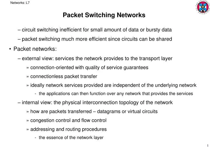
Packet Switching Networks. circuit switching inefficient for small amount of data or bursty data packet switching much more efficient since circuits can be shared Packet networks: external view: services the network provides to the transport layer

E N D
Networks: L7 Packet Switching Networks • circuit switching inefficient for small amount of data or bursty data • packet switching much more efficient since circuits can be shared • Packet networks: • external view: services the network provides to the transport layer • connection-oriented with quality of service guarantees • connectionless packet transfer • ideally network services provided are independent of the underlying network • the applications can then function over any network that provides the services • internal view: the physical interconnection topology of the network • how are packets transferred – datagrams or virtual circuits • congestion control and flow control • addressing and routing procedures • the essence of the network layer
Networks: L7 • Possible network services: • best-effort connectionless, low-delay connectionless • connection-oriented reliable stream service, packet transfer with delay and bandwidth guarantees • End-to-End services versus Hop-by-Hop services • end-to-end argument suggests functions should be placed at the edges of the network • the application is in the best position to determine whether a function is being carried out completely and correctly • as much functionality as possible located in the transport or higher layers • on this basis, the network layer should only provide the minimum needed to meet the required application performance • keeps network simple and enhances scalability to very large networks • functions necessarily hop-by-hop include • packet routing and forwarding, priority and scheduling of packets • congestion occurs within the network level but may require action at the edge level to reduce flows
Networks: L7 • Packet Network Topology • Local Area Networks (LANs) to Wide Area Networks (WANs) Gateway Organization Servers To Internet or ISP s s Campus Backbone R R Backbone Switches R S Departmental Server S S R R R s s s LAN Switch s s s s s s
Networks: L7 • LANs allow sharing of resources such as printers, databases, software • extended LANs or Virtual LANs over physical LANs and LAN switches • reconfigurable by software • contains the amount of traffic using the organisation’s network • LANs linked into Campus networks via a backbone network • organisation servers and databases • with redundant links to the backbone • gateways to outside world • the Internet, ISPs etc. • Campus networks joined into metropolitan area networks • e.g. EastMan – the Edinburgh and Stirling network • http://www.eastman.net.uk • National networks • JANET – the Joint Academic Network for UK Higher Education institutions • http://www.ja.net
Networks: L7 • routers in a campus network or national academic network form a domain or Autonomous System • with Border routers to the outside world • separate routing protocols within domains and between domains Interdomain level Border routers Autonomous system or domain Border routers LAN level Intradomain level
Networks: L7 • Connectionless Packet Switching • the network does not need to be informed of a flow ahead of time • no prior allocation of network resources • just two basic interactions with network level • a request to send a packet • an indication that a packet has arrived • responsibility for error control, sequencing, flow control placed entirely on the end-system transport layer • derived from message switching systems • messages relayed from switch to switch in store-and-forward fashion Message Message Message Subscriber A Message Subscriber B Network nodes
Networks: L7 Source T t Switch 1 t p Switch 2 t t Destination Delay • message switching can achieve a high utilisation of the transmission line • but delay over multiple hops can be long : • whole message has to be received before it can be transmitted on • minimum delay = 2p + 3T, assuming equal speed lines and no queueing delay • probability of transmission error also increases with length of the block • e.g. message length L = 106 bits over two hops with error rate p = 10-6 and each hop doing error checking and retransmission • probability of message arriving correctly = (1-p)L = (1-10-6)1000000 1/3 • i.e. about three tries for each hop • 6 Mbits transmitted in total to get message across
Networks: L7 Packet 1 Packet 1 Packet 2 Packet 2 Packet 2 • long messages may hold up other traffic waiting for the line for long periods • not suitable for interactive traffic • like a non-preemptive scheduler and a CPU-bound job in Operating Systems • long messages therefore need to be broken up into smaller packets • a limit on maximum packet size limits maximum delay for other waiting packets • in connectionless packet-switching, each packet (datagram) is routed independently through the network : • in practice may well take the same route • but may not depending on link and switch failure, congestion etc.
Networks: L7 • at each switch the final destination address is extracted from the header • and used in a look-up table to determine the forwarding output port : • when the size of the network becomes large, a route look-up algorithm needs to be used in place of table indexing • routing tables updated dynamically when network failures occur • by adjacent switching nodes sharing information • datagram routing therefore robust • the same routing nodes do not need to be available for the whole message Output port Destination address 0785 7 1345 12 1566 6 2458 12
Networks: L7 Node 3 Destination Next node Node 6 Node 1 Destination Next node 1 1 Destination Next node 2 4 1 3 2 2 4 4 1 2 5 3 3 3 5 6 3 3 4 4 6 6 6 4 3 5 2 5 5 A 6 3 Node 4 4 B Destination Next node Host 1 1 2 2 2 Node 2 Node 5 Switch or router 5 3 3 Destination Next node Destination Next node 5 5 1 1 1 4 6 3 3 1 2 2 4 4 3 4 5 5 4 4 6 5 6 6 • network example:
Networks: L7 Source t 1 3 2 p Switch 1 t 3 1 2 p + P Switch 2 t p + P 1 2 3 t L hops 3 hops Lp + (L-1)P first bit received 3p + 2(T/3) first bit received Lp + LP first bit released 3p + 3(T/3) first bit released 3p + 5 (T/3) last bit released Lp + LP + (k-1)P last bit released where T = k P • delay incurred by messages broken into separate packets: • e.g. three packets following the same path are transmitted in succession : • now only have to wait until first packet arrives before it can be forwarded • Internet Protocol (IP) an example of connectionless packet transfer
Networks: L7 Connect request Connect request Connect request SW 1 SW n SW 2 … Connect confirm Connect confirm t Connect request 1 3 2 CC t Release 3 CR 1 2 CC t Connect confirm CR 1 2 3 t • Connection-oriented packet switching : Virtual Circuits • network layer must be informed about the upcoming flow ahead of time • transport layer cannot send information until the connection is set up • set up parameters may be negotiated: level of usage, Quality of Service, network resources • message exchanges between each segment of the route through the network: • extra delay overhead for setting up the virtual circuit : • a release procedure also required to terminate the session
Networks: L7 • the same path is used for all packets • more vulnerable to network failure • all the affected connections must be set up again • resources can be allocated during connection set up • number of buffers • amount of guaranteed bandwidth • the individual links are still shared by many separate packet flows • the number of flows admitted may have to be limited • to control congestion and ensure that switch can handle the volume of traffic • when delays or link utilisation exceed a certain threshold • network has to maintain state information about the flows it is handling • can grow large with numerous virtual circuit flows
Networks: L7 Source t 2 1 3 Switch 1 t 2 3 1 Switch 2 t 2 1 3 t Destination • minimum delay for transmitting a message normally the same as before • but a modified form, cut-through packet switching possible • where retransmissions not used in the underlying datalink control • packets are forwarded as soon as the header arrives and the table lookup is carried out • reduces the minimum delay by overlapping packet transmissions • appropriate for applications such as speech transmission • where there is a maximum delay requirement • and some errors tolerable • also appropriate for virtually error-free transmission lines e.g. optical fibre • hop-by-hop error checking unnecessary
Networks: L7 • Virtual Circuit Identifiers (VCIs) • datagram packets must contain the full address of source and destination • significant number of bits e.g. 128bits in IPv6, and resultant packet overhead • in virtual-circuit switching, abbreviated headers can be used • in connection set up, entries are added to forwarding, or routing, tables • at input to each switch, connection can now be identified by a VCI • only need a smaller range of numbers (and fewer bits) just for the virtual circuits that go through this switch • a significant advantage of virtual circuit switching over datagrams • the VCI used to index into the routing table: Output port Next identifier Identifier 12 44 13 Entry for packets with identifier 15 15 15 23 27 13 16 58 7 34
Networks: L7 2 7 1 8 B 1 3 3 A 1 6 5 5 4 2 4 3 5 2 C 5 6 D 2 • hardware-based table look-up allows fast processing and packet forwarding • datagrams routing typically need a search algorithm to find next hop • entry can also specify a priority for packets in this flow • table entry for a VCI can also specify the VCI to be used for the next hop • the next switch in the route may have a different set of virtual circuits going through it and different VCIs • local rather than global VCIs require fewer bits in the header • only the maximum VCI number in any switch • searching for a spare VCI number is simpler – only local to the switch • Example: • virtual circuit path from A to B uses VCIs 1, 2, 7, 8 in successive links • virtual circuit path from A to D uses VCIs 5, 3, 4, 5, 2 etc.
Networks: L7 Node 3 Incoming Outgoing Node 6 Node 1 node VC node VC 1 2 6 7 Incoming Outgoing Incoming Outgoing 1 3 4 4 node VC node VC node VC node VC 4 2 6 1 3 7 B 8 A 1 3 2 6 7 1 2 3 1 B 5 A 5 3 3 6 1 4 2 B 5 3 1 3 2 A 1 4 4 1 3 B 8 3 7 3 3 A 5 Node 4 Incoming Outgoing node VC node VC 2 3 3 2 Node 2 Node 5 3 4 5 5 Incoming Outgoing Incoming Outgoing 3 2 2 3 node VC node VC node VC node VC 5 5 3 4 C 6 4 3 4 5 D 2 4 3 C 6 D 2 4 5 • corresponding routing table at each switch:
Networks: L7 R2 R2 R1 R1 • Hierarchical Routing • size of routing tables can be reduced if addresses allocated hierarchically • hosts near to each other should have addresses with a common prefix • routers then only need to examine part of the address to decide routing: • instead of: • e.g. IP network, subnetwork and host addresses 0100 0101 0110 0111 0000 0001 0010 0011 1 4 3 5 2 1100 1101 1110 1111 1000 1001 1010 1011 00 1 01 3 10 2 11 3 00 3 01 4 10 3 11 5 0001 0100 1011 1110 0000 0111 1010 1101 1 4 3 5 2 0011 0110 1001 1100 0011 0101 1000 1111 0001 4 0100 4 1011 4 … … 0000 1 0111 1 1010 1 … …
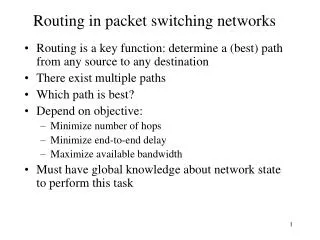
Networks: L7 • Routing in Packet Networks • an objective function needed to determine the best route • e.g. minimum number of hops, minimum end-to-end delay, path with greatest available bandwidth etc. • algorithms should seek certain goals: • rapid and accurate routing • must quickly be able to find a route if one exists • adaptability to network topology changes • due to switch or link failures • must be able quickly to reconfigure routing tables • adaptability to varying loads • loads over certain routes change throughout the day • must be able to reconfigure best according to the current loads • ability to route packets away from temporarily congested links • load balancing over links desirable • ability to determine connectivity of the network • to be able to find optimal routes • low overhead of control message interchange between routers
Networks: L7 • Algorithm Classification • static routing • network topology initially determined and remains fixed for long periods • may even be manually set up and loaded into routing tables • inconvenient for large networks • unable to react quickly to network failures • the larger the network the more likely failures and changes in topology • dynamic (or adaptive) routing • each router continually learns the state of the network • by communicating with its neighbours • a change in network topology is eventually propagated to all routers • each router can then recompute the best paths and update its tables • but adds to the complexity of the router • routing can be decided on a per packet basis for connectionless transfers • cannot make use of its adaptability for virtual circuit transfers • fixed once the connection set up
Networks: L7 • centralised routing • a network control centre computes all routing paths • uploads the information to all the routers • allows individual routers to be simpler • vulnerable to a single point of failure • distributed routing • routers cooperate by means of message exchange • perform their own routing determinations • scale better than centralised schemes • may react more quickly to local network failures • just need to use local information to reroute around a failure • instead of propagating the change information right back to the control centre • more likely to produce inconsistent results • e.g. A thinks best route to Z is through B; B thinks best route to Z is through A • packets may get stuck in a loop
Networks: L7 • shortest path algorithms invariably used to find best routes • according to some weighting metric • distance vector routing: • neighbouring routers exchange routing tables with the set, or vector of known distances to other destinations • routers process this to find better routes through the neighbour • and adapt to changes in the network topology as information percolates through the network • e.g. Bellman-Ford algorithm, RIP and BGP Internet protocols • link state routing: • each router broadcasts information about the state of its links to neighbours and other routers pass this information on further • each router can therefore construct a map of the entire network • and from this derive a routing table • e.g. Dijkstra’s algorithm, OSPF Internet protocol • RIP and OSPF-2 : Interior Gateway Protocols, used within Autonomous Systems • BGP-4 : the current Exterior Routing Protocol between Internet AS’s
Networks: L7 • Dijkstra’s algorithm • iterative scheme successively finding closest nodes to source • 1st iteration: find neighbouring node closest to source • 2nd iteration: find next closest node • either a neighbour of the source • or a neighbour of the closest node found in the 1st iteration • 3rd iteration: next closest • either a neighbour of the source • or a neighbour of the nodes found in 1st or 2nd iterations • etc. • on the kth iteration, the algorithm will have determined the k closest nodes • continues until all nodes are covered • let N be a set of permanently labelled nodes • nodes whose shortest paths from source have been determined • with s the source node • let Di be the current minimum cost from source to node i • let Cij be the cost of the path from node i to node j
Networks: L7 1. Initialisation: N = {s} Dj = Csj j s ( = if no direct connection) Ds = 0 2. Finding next closest node: find node i Nsuch that Di = min Dj , j N add i to N if N contains all nodes, stop 3. Updating minimum costs: for each node j N , Dj = min { Dj , Di + Cij } Goto step 2
Networks: L7 2 1 1 3 6 5 2 3 2 4 1 1 3 1 2 3 6 2 2 5 4 3 4 2 2 5
Networks: L7 2 1 1 3 6 5 2 3 4 1 2 3 2 5 4 • Bellman-Ford algorithm • intuitively, if a node is on the shortest path between nodes A and B • the path from the node to A must be the shortest path • and the path from the node to B must also be the shortest path • example: • to find shortest path from node 2 to node 6: • packet from node 2 must go through node 1, node 4 or node 5 • if shortest path from nodes 1, 4, 5 are 3, 3, 2 respectively, • from node 2: • total cost through node 1 is 6; through node 4 is 4; through node 5 is 6 • so shortest path from 2 to 6 should go through node 4
Networks: L7 • let Djbe the current estimate of the minimum cost from node j to the destination node d • let Cij be the cost from node i to node j • Cij= 0 if i= j ; Cij = if i and j not directly connected 1. Initialisation: Di = , i dDd = 0 2. Updating: for each i d , Di = min { Cij + Dj } j i Repeat step 2 until no more changes occur • will eventually converge since initially Di = for all i • and at each iteration, Di are non-increasing and bounded below
Networks: L7 2 1 1 3 6 5 2 3 4 1 2 2 1 3 1 3 2 6 5 2 4 4 1 2 2 5 • example, shortest paths to node 6: • label each node i with (n, Di) • where n is the next node along the current shortest path ( = -1, if not defined)
Networks: L7 • Bellman-Ford lends itself to a distributed implementation • each node independently recomputes its minimum cost to each destination: Dii = 0Dij = min { Cik + Dkj }k i • and periodically broadcasts its vector of costs { Di1, Di2, Di3 … } to its neighbours • a change of routing table can trigger a node to broadcast • this allows routing tables to adapt to changes in network topology • Recomputing Minimum cost : example: • a broken link from node 3 to node 6 • as soon as node 3 detects that the link to 6 is broken, it recomputes the minimum cost to node 6 • and finds that the new minimum is 5, via node 4 • since node 4 still thinks its minimum cost route is 3, via node 3 ! • then node 3 sends a routing update to its neighbours, nodes 1 and 4 • nodes 1 and recompute their costs and broadcast, node 3 rerecomputes etc.
Networks: L7 2 1 3 X 6 5 2 3 4 2 1 3 2 5 4
Networks: L7 1 2 3 4 X 1 1 • Reaction to link inaccessibility: • suppose link 3-4 breaks • accessibility to node 4 : • each link keeps updating its cost in increments of 2 • at each iteration, node 2 thinks shortest path is through node 3 • and node 3 thinks shortest path is through node 2 • messages bounce backwards and forwards • the counting to infinity problem, in practice until some threshold is reached
Networks: L7 • several approaches to dealing with counting to infinity problem • split horizon : • minimum cost to a given destination is not sent to a neighbour if that neighbour is the next node along the shortest path • e.g. if node X thinks best route to node Y is through node Z, then X should not send the corresponding minimum cost to Z • stops the bouncing to and fro of previous example • split horizon with poisoned reverse : • allows a node to send the minimum costs to all its neighbours • but the minimum cost to a given destination is set to infinity if the neighbour is the next node along the shortest path • e.g. if node X thinks best route to node Y is through node Z, the node X should set the corresponding minimum cost to infinity before sending it to Z • again stops bouncing to and fro
Networks: L7 • previous example using split horizon with poisoned reverse : • Java Applet simulation of of Bellman-Ford downloadable from: http://www.laynetworks.com/users/webs/bellmansimulation.htm
Networks: L7 • Flooding • in principle: each switch forwards incoming packets to all ports • except the one the packet was received from • the packet will eventually reach the destination if a route exists • very inefficient in general but • useful when routing information not available • e.g. at system start up • when survivability is required • e.g. in military systems • also effective when source needs to broadcast to all hosts in the network • unfortunately flooding may swamp the network with an exponentially increasing number of packets • possible solutions: • a time-to-live field set to some small number, decremented at each switch and the packet discarded when the count reaches zero • initial value could be set to the minimum hop distance between the two nodes furthest apart – the diameter
Networks: L7 1 3 6 4 2 5 1 3 6 4 2 5 1 3 6 4 2 5 • example: time-to-live flooding with a network diameter of 2 : (a) (b) (c)
Networks: L7 • second possibility: • each switch adds its identifier to the packet header before it floods • when a switch encounters a packet with its own identifier, it discards the packet • prevents packet going round in a loop • third possibility: • similar to previous method – both try to discard packets • each packet from a given source is identified with a unique sequence number • when a switch receives a packet, it records the source address and the sequence number • if that packet has already visited that switch it is discarded • all possibilities require extra header information • 3rd requires switch to store considerable amount of extra information also
Networks: L7 0,0 0,1 0,2 0,3 1,0 1,1 1,2 1,3 2,0 2,1 2,2 2,3 3,0 3,1 3,2 3,3 • Deflection routing • when forwarding a packet, if the preferred port is not available • e.g. busy or congested • packet is deflected to another port • works well in a network with a regular topology • example: a Manhattan network: • switches identified by a row and column number • unidirectional ports in this case
Networks: L7 busy 0,0 0,1 0,2 0,3 1,0 1,1 1,2 1,3 2,0 2,1 2,2 2,3 3,0 3,1 3,2 3,3 • to send a packet from switch (0, 2) to switch (1, 0) : • packet could go via switches (0, 1) and (0, 0) • if left port of (0, 1) is busy, packet will be deflected to (3, 1) • and then through switches (2, 1), (1, 1), (1, 2), (1, 3) to (1, 0) : • advantage: the switches can be bufferless • packets do not need to wait for the preferred port to be available • useful in an all optical network • or in very high speed switches where buffering is expensive • since alternative paths can be taken, in-sequence delivery not guaranteed
Networks: L7 1,3,6,B 3,6,B 6,B 1 3 B 6 A 4 B Source host 2 Destination host 5 • Source routing • does not require intermediate nodes to maintain routing tables • source host has to know the precise path through the switches to be used • this sequence of nodes is included in the packet header • and gives each node sufficient information to know how to forward an arriving packet • each node strips off the label identifying itself and forwards the packet to the node indicated by the next label
Networks: L7 • works for both datagrams and virtual-circuit packet switching • the complete route can be preserved as the packet passes through the switches • an extra pointer or counter field incorporated to identify the next node • updated as the packet passes through each switch • this allows the destination to send replies back over the reverse path • by reversing the order of nodes in the path in the header • useful for monitoring the switches in the path • Internet Protocols IPv4 and IPv6 provide an option for source routing