Download
1 / 46
460 likes | 662 Views
Chapter 7 Packet-Switching Networks. Dept of computer science and engg 6 th sem cse SSE. Virtual circuit packet switching. Virtual circuit packet switching establishes a fixed path called VIRTUAL CIRCUITS.

E N D
Chapter 7Packet-Switching Networks Dept of computer science and engg 6th sem cse SSE
Virtual circuit packet switching • Virtual circuit packet switching establishes a fixed path called • VIRTUAL CIRCUITS
VIRTUAL CIRCUIT SETUP PROCEDURE will take place before any packets flow through the network. • Virtual circuit resides in network layer. Figure 2 • Delay is incurred when a message is broken into 3 packets and transmitter over the circuit. • Same delay as datagram packet switching execpt for additional delay used to set up the circuit.
Path is determined parameters are set in swiches by exchanging Connect request and Connect confirm messages • If the switch does not have enough resources then it responds with a connect reject message and the setup procedure fails. • Figure 3 • At the input of every switch ,the virtual circuit is identified by • VIRTUAL CIRCUIT IDENTIFIER(VCI)
When packet arrives at the input port the VCI in the header is used to access the table. • The table lookup provides the output port to which the packet is fowarded and the VCI that is used at the input port of the next switch. • Call setup procedure sets up chain of pointers across the network that directs the flow of packets • Figure 4
Structure of packet switch • A packet switch will perform two main functions • ROUTING • FORWARDING • Routing function uses algorithm to find path to destination • Stores result in routing table • Forwarding function processes incoming packet from input port • Forwards packet to appropriate output port based on routing table information
Generic packet switch • Input port, output port, interconnection fabric, switch controller
Input ports and output ports are paired Line card • Contain several input/output port. • Capacity of link connecting the fabric is high speed, fully utilized • Implements physical, data link and network layer functions • Symbolic timing, line coding, framing, physical layer addressing ,error checking
Organization of line cardmade up of various chipset Figure 6-> • Line card supports medium access control protocol to handle broadcast network. • Implemented by special purpose chipset • Network layer routing table in line card • Need to perform fast table lookup to find output port • Contain buffers and associated scheduling algorithms • Network processor performs table lookup and packet scheduling
Controller • Contain general purpose processor • This manages control and management functions • If controller is connectionless executes routing protocol • If connection oriented handles signally messages. • Controller communicates with line card and fabric to configure internal parameters.
Inter connection fabric • Transfers packet between line card • Crossbar interconnection fabric transfer packets parallel between input and output ports • Buffers are added to crossbar to accommodate packet contention. • Buffer located at input or output port.
Output buffering • Crossbar with output buffering should run N times faster than port speed as N packets simultaneously arrive at a particular output • If output is idle, one packet is transmitted rest are buffered. • Only one packet is allowed to proceed to particular output
Input buffering • 2 packets at input 2,first packet like to go to output 3,second to output 8 • Packet from input buffer 1 also want to go to output 3 • Frist packet from input buffer should wait ,2nd should wait behind 1st even though output 8 is idle • Results in performance degradation . • Problem called HEAD of Line Blocking
Banyan switch • Solution is building a large switch • Composed of 2*2 switching elements interconnected in certain fashion` • Exactly 1 path will exist from input to each output • Routing is done in distributed manner • Ie appending binary the binary address of the output number to each packet • Switching element at stage I steers a packet based on ith bit of the address. • Bit is 0 the element steers packet to upper output.
Input 1 likes to send it to the output destines to packet 5 • The switching element at stage 1 looks at first bit Of the address and steers the packet to its lower output. At stage 2 it steers the packet to the upper output since the second bit is 0.at stage 3 steers the packet to lower output and sends to output 5
Routing in packet networks • Routing is concerned with determining feasible paths for packet to follow from source to destination 1)Rapid and accurate delivery of packets Routing algorithm should operate correctly Find path to correct destination Should not take long time to find path 2)Adaptablilty to changes in network topology Network equipment and transmission line will fail Routing algorithm should adapt and reconsider the path. 3)Adaptability to various source destination traffic loads Traffic loads change dynamically, hence should adjust path based on the current traffic loads.
4) Ability to route packets away from congested links Routing algorithm should avoid congested links and balance the load. 5) Ability to determine connectivity of network Routing system should know connectivity to find optimal paths 6)Ablility to avoid loops Inconsistent information will lead to routing loops. Routing system should avoid the loops in presence of distributed routing system. 7)Low Overhead Should obtain connectivity information by exchanging control messages with routing system. These messages create overhead on bandwidth usage and hence should be minimized.
Routing algorithm Classification • Routing algorithm is classifies as • 1) Static routing • 2)Dynamic routing Static routing Paths are precomputed based on the network topology, link capacities and other information Computation is completed the paths are loaded in the routing table of each node. This remains fixed for a long time. Works when network size is small, and the traffic doesn’t change in time It becomes cumbersome, as network size increases. Disadvantage is inability react to network failures
Dynamic routing • Each node will continuously learn the state of the network by communicating with the neighbors • Change in network topology is eventually propagated trough nodes • Based on the information the node computes the best path to the destination • Disadvantage is the added complexity with the nodes. • They can also be distinguished as • Centralized routing • Distributed routing
Centralized and Distributed routing • In Centralized routing the network control center computes all the path and then uploads the information in the network • In Distributed routing nodes cooperate by the means of message exchanges and perform their own routing computations. • Distributed routing is better than centralized routing but generate inconsistent results ,loop wil develop • If A thinks B is the best path to Z and If B thinks A is the best path to B • Then desired packet to Z have the misfortune of arriving at A or B and stuck in a loop between A and B
Routing Tables • Once the routing algorithm defines the set of path the path information is stored in the routing table. • In virtual circuit packet switching the routing table translates each incoming VCI to outgoing VCI an identifies the output port to which the packet is to be forwarded. • Datagram packet switching the routing table identifies the next hop to forward the packet based on destination address of the packet • Virtual circuits are bidirectional.
A packet sent by node A with VCI 1 will eventually reach node B and from node A with VCI 5 will reach node D VCI 1 from node A will be translated to 2 and to 7 and finally to 8 and reaches B When node 1 will receive the header with VCI 1 that node replaces the incoming VCI with 2 ande forwards the packet with node 3
If a packet with VCI 5 arrives at node 1 from node A,the packets is forwarded to node 3 after the VCI is replaced with 3 • After arriving at node 3 the packet receives the outgoing VCI 4 and is forwarded to node 4 • Node 4 translates the VCI to 5 and forwards the packet to node 5. • Node 5 translates to VCI 2 and delivers the packet to destination node D • The routing table uses node numbers to identify where the packet comes from and where the packet is forwarded.
Shows routing table for network topology • Minimum hoping routing objective • Packet destines to node 6 arrives at node 1, the packet is fowarded to node 3 based on the corresponding routing table entry • Node 3 forwards the packet to node 6
Hierarchical routing • The size of routing table is reduced • Hosts that are near to each other should have addresses that have common perfixes • Routers will examine the part of address and decide to route the packet • Example of hierarchal address assignment and flat address assignment
flooding • Forwards an incoming packet to all the ports except the one received from • Each switch performs the flooding process and eventually reach the destination • Effective routing approach when the routing information is not available • Also effective when source need to send packet to all the nodes • Flooding may easily swamp network
To reduce resource consumption in the network • Time to live field (TTL) in each packet • Source sends the packet TTL is set to some number • Each node decrements the TTL by 1 before flooding the packet • If value reaches 0 the node discards the packet • Avoid wastage of bandwidth, minimum hop number between two further nodes • 2nd ,the node adds identifier to header of packet • When node receives the packet that contain the identifier it discards it as it knows packet already visited the node(prevents looping) • Identified with unique sequence number,node will record the sequence number and source address • If already visited it will discard the packet
Deflection routing • Also called hot potato routing. eg: Manhatten street network • They provide multiple path for each source –destination • Each path tries to forward the packet to the preffered port • If preferred port is busy or congested the packet is deflected to another port
Advantage is node are buffer less, packets do not have to wait for a specific port to become available • If unavailable it will deflect the packet to another port, reaches destination • Since they take alternate path they cannot guarantee in-sequence delivery of packets • Used in optical network where optical buffers are difficult to find • Used to implement high speed switches where topology is regular and buffers are expensive
Shortest path routing • Routing algorithm is based on Shortest path algorithm • Each link represents the cost of using the link • Shortest path between node 2 to node 6 is trough 2-4-3-6 and the cost path is 4 Metrics used to assign the cost • Cost ~ 1/capacity : Higher cost to lower capacity links • Cost ~ packet delay: It includes queuing delay in switch buffer and propagation delay in link 3 Cost ~ Congestion : Congestion measure is traffic loading. Avoids Congested link
The Bellman – Ford Algorithm • If Neighbor of node A knows the shortest path to node Z ,then node A can determine the shortest path to Z • Ie Node A will calculate the cost/Distance to node Z trough its neighbors by picking the minimum
Dj – Current estimate to minimum cost to destination node • Cij – link cost from node I to node j (c13=c31=2) (c11=0) (c15=c23= ∞) Minimum cost from node 2 to node 6 trough node 1 ,node 4 and node 5: D2= min{C21 + D1 , C24 + D4 ,C23+ D5} = min{3+3,1+3,4+2} =4 1.Initialization: Di= ∞ for all i ≠ d Dd=0 2. Updating: for each I ≠d Di= Minj {Cij + Dj} for all j ≠ i
Initally all the nodes other than the destination node are at infinite cost to node 6. • (Iteration 1)Node 3 finds that it is connected to node 6 with cost of 1.Node 5 finds it is connected to node 6 with cost 2.Node 3 and 5 update their entries. • (Iteration 2)Node 1 finds it can reach node 6 via node 3 with cost 3.Node 2 finds it can reach node 6 via node 5 with cost 6. Node 4 finds it has path via 3 and 5 with costs 3 and 7 respectively.Node 4 selects the path via node 3.Node 1,2 and 4 update their entries • (Iteration 3)Node 2 finds it can reach node 6 via node 4 with distance 4.Node 2 changes the entry to (4,4) and informs the neighbours • Node 1,4,5 processes the new entry from node 2 but donot find new shortest paths.The algorithm is conservged
Link connecting node 3 and node 6 breaks. Compute minimum cost for each node to destination node.
(update 1)As soon as node 3 detects that link(3,6) breaks, node 3 recomputed the minimum cost to node 6.Node 3 looks for path to 6 trough neighbours, Node 1 and Node 4 and its calculation indicates that the new shortest path is trough node 4 at a cost of 5.Node 3 then sends the new routing updates that is node 1 and node 4 • (update 2)Node 1 and 4 recomputes their minimum costs; node 1 findsits shortest path is still trough node 3 but the cost has increased to 7;node 4 finds the shortest path is trough node 2 or node 5 with cost 5.node 4 chooses node 2.Node 1 transmits its routing updates to node 2,node 3 and node 4 • Node 4 transmits its routing updates to node 1,2,3,5
(Update 3)Node 1 finds its shortest path is still trough node 3.Node 2 finds its shortest path is still trough node 4 but the cost has increased to 6.Node 3 finds its shortest path is still through node 4 but the cost has increased to 7.Node 4 and Node 5 finds the shortest path is not changed. Node 2 transmits its updates to node1,node4 and node 5 and transmits its updates to node 1 and 4. • (update 4) Node 1 finds its shortest path is through either node 2 or node 3 with cost 9.Suppose that node 1 chooses node 2.Node 4 now finds the shortest path through node 5 with cost 5 since the cost through 2 has incresed to 7.Node 5 does not change its shortest path.Node 1 transmits its updates to node 2,node 3,node 4 and node 4 transmit its updates to node 1,2,3 and 5 • (update 5) None of the nodes find short paths
Update node1 node2 node3 Before break (2,3) (3,2) (4,1) After break (2,3) (3,2) (2,3) • (2,3) (3,4) (2,3) • (2,5) (3,4) (2,5) • (2,5) (3,6) (2,5) • (2,7) (3,6) (2,7) • (2,7) (3,8) (2,7)
Split Horizon with poison reverse • Update Node 1 Node 2 Node3 Before break (2,3) (3,2) (4,1) After Break (2,3) (3,2) (-1, ) 1 (2,3) (-1, ) (-1, ) 2 (-1, ) (-1, ) (-1, ) After the link breaks node 3 sets the cost of the destination to infinity,since the minimum cost node 3 has received from node 2 is also infinity.When node 2 received the update message it also sets to infinity.Node 1 learns the destination is unreachable
Dijkstra ‘s Algortihm • Alternate algorithm for finding the shortest paths to source to all other nodes. • To identify the closest nodes from the source node in the order of their increasing path cost. • 1 Initialalization N={s} Dj=Csj,for all j ≠ s 2.Finding the next closest node Di=min Dj Add i to N 3.Update minimum cost from node I to node N Dj=min{Dj,Di+Cij}
Source routing versus Hop by Hop Routing • Datagram network each node determines the next hop along the shotest path ,packet travels from source as it follows HOP BY HOP routing to destination • SOURCE ROUTING the path to the destination is determined by source.Explicit routing allow a perticular packet node to determine the path. • Source includes path information in the packet header that contain sequence of nodes to traverse and sufficient information to nodes till packet is fowarded to destination.
Each node examines the header,removes address identifying the node,forwards packet to next node • If we reserve the path information we can traverse the node back to the source by reversing the path.
Link state routing versus Distance vector routing • Distance Vector routing Neighboring routes exchange routing tables that sets the vector of known distance to destination. Bellman ford algorithm is used to find the best path though information from the neighbors. With new path the router wil send new vector to neighbors. This adapts to change in network topology Link State Routing Each router will flood information to the state of the links that connects to neighbors Allows routers to construct map of entire network and then uses Djikstra s algorithm. If state is changed the router detects the change and floods the new information to network
ATM Networks • Asynchronous transfer mode (ATM) is a method for multiplexing and switching that supports broad range of services • Connection oriented packet switching technique that provides quality of service(QoS) • Variable bit rate delay bursty traffic processing • TDM Multirate only low,fixed Inefficient Minimal ,high speed • Packet Easily handled variable efficient header and packet processing
ATM is packet based,can easily handle services and generate information in bursty fashion on variable bit rates. • The abbreviated header of ATM facilitates implementations that result in low delay and high speed
Information flow generated from various users is converted into cell and sent to ATM multiplexer • It arranges the cell into one or more queues and implements some scheduling strategy to determine which order it is transmitted