Download

1 / 27
270 likes | 364 Views
Adjustment of Global Gridded Precipitation for Orographic Effects. Jennifer C. Adam 1 Elizabeth A. Clark 1 Dennis P. Lettenmaier 1 Eric F. Wood 2. Dept. of Civil and Environmental Eng., University of Washington Dept. of Civil Eng., Princeton University. precipitation divide.

E N D
Adjustment of Global Gridded Precipitation for Orographic Effects Jennifer C. Adam 1 Elizabeth A. Clark 1 Dennis P. Lettenmaier 1 Eric F. Wood 2 • Dept. of Civil and Environmental Eng., University of Washington • Dept. of Civil Eng., Princeton University
precipitation divide increased condensation and precipitation due to orographic lifting decreased precipitation: the “rain shadow” Motivation: The Orographic Effect on Precipitation * No global gridded precipitation datasets take into account the effects of orographic lifting Figure taken from http://jamaica.u.arizona.edu
PRISM (Daly et al. 1994, 2001, 2002)(Parameter-elevation Regressions on Independent Slopes Model) • 2.5 minute • Topographic facets • Regresses P against elevation on each facet 0 100 200 300 400 500 mm/month
Basin Area/Station Location Distributions Station Count Basin Area 100% Africa 20% 100% Asia Cumulative Percent 20% 100% Australia 20% 100% Europe 20% 100% North America 20% 100% South America 20% 0.5 1.0 1.5 2.0 2.5 Elevation, km
Stream Flow Simulations 15,000 400 800 1200 1600 Precipitation, mm/year 10,000 5,000 0 m3/s J F M A M J J A S O N D Observed with GPCC precipitation with PRISM precipitation 2°×2° GPCC 1/8°×1/8° PRISM 2°×2° PRISM From Nijssen et al. 2001 (J. Clim.)
Objectives • Consistent framework to account for orographic effects in 0.5° gridded gauge-based precipitation estimates on a global scale • Utilize existing gridded precipitation product: Willmott & Matsuura (2001) with correction for precipitation under-catch by Adam & Lettenmaier (2003). • Mean annual correction for 1979-1999
Outline of Steps • Definition of Correction Domain (regions of complex topography, only) • Average Correction Ratio for Gauged Basins: the “Budyko Method” • Fine-Scale Spatial Distribution of Correction Ratios within Gauged Basins • Fine-Scale Interpolation of Correction Ratios to Un-Gauged Basins then aggregate to 0.5° Step 1 Step 2 Step 3 Step 4
Select Correction Domain Step 1 • Pre-selection according to slope: • - slopes calculated from 5-minute DEM • - aggregated to half-degree • 2. Set Slope Threshold • 6 m/km (the approximate slope above which Willmott & Matsuura (2001) differs by more than 10% from PRISM) • 3. Final Domain – smoothing then final selection
Slope, m/km 0 5 10 15 20 25 30 35 40
Step 2 Basin-Average Correction Ratios: the “Budyko Method” • 1. Determine “actual” basin average precipitation by solving 2 simultaneous equations: • Water Balance equation: • Derivative of Budyko (1974) E/P vs. PET/P curve • 2. Calculate average correction ratio for each basin:
Moisture Limited Energy Limited Budyko (1974) Curve S&V: Sankarasubrumanian and Vogel (2002) Uses an additional parameter: soil moisture storage capacity
Gauged Basins 357 mountainous basins chosen
Spatial Distribution of Correction Ratios Within Gauged Basins Step 3 • Break correction domain into a 5-min grid of “correction bands” – gives degree of topographic influence • Spatially distribute: use quadratic equation • B, C: from constraints, i.e. (Rave conserved over basin and rband unity outside correction domain) • A: from regressing Rave with PRISM (developed using 101 basins in western North America, tested over 5 basins in central Asia)
1 2 3 4 5 6 e.g. San Joaquin, CA Correction Bands Elevation, m Correction Ratio
Interpolate to Un-Gauged Areas Step 4 • Interpolation at 5-min resolution: uses a linear distance weighting scheme • Only interpolates to cells with the same correction band and the same slope type (i.e. windward vs. leeward – determined from NCEP/NCAR reanalysis data) • 2. Aggregate 5-min correction ratios to the final resolution – 0.5° • 3. Apply to original data via multiplication
Results 0.4 0.8 1.2 1.6 2.0 Correction Ratio
Summary • Satisfies a need for gridded precipitation data that account for orographic effects in a globally-consistent framework • Uses combination of water balance and Budyko (1974) curve to get magnitude, PRISM used to help derive spatial variability • Final product: 1979-1999 0.5° climatology that accounts for gauge under-catch and orographic effects (global increases are 11.7% and 6.2%, respectively, for a net of 17.9%)
Increases with Elevation 100% Africa 100% Percent Increase Australia 100% Eurasia 100% North America 100% South America 100% Globe 0 1 2 3 4 5 6 km
Percent Increase Implied PRISM Adjustments (as compared to Willmott&Matsuura 2001) Net: 13.6%, 35.5% Cv = 1.41 Adam et al. Adjustments Net: 16.1%, 41.6% Cv = 0.42
Further PRISM Comparisons Adam et al. PRISM
Least Topographic Influence Most Topographic Influence 1 3 5 2 4 6 Correction Bands
Upslope Downslope Cross-Wind Slope Type
Where = Aridity Index Where = Soil Moisture Storage Index = Soil Moisture Storage Capacity Equations 1 2
Water Balance In General: Long term mean over watershed: “Q” obtained from streamflow measurements
Distributions with Elevation Station Density Area 20% Africa Percent per Elevation Increment 20% Asia 50% Australia 20% Europe 20% North America 20% South America 0 0.5 1.0 1.5 2.0 2.5 km