Download
1 / 9
90 likes | 183 Views
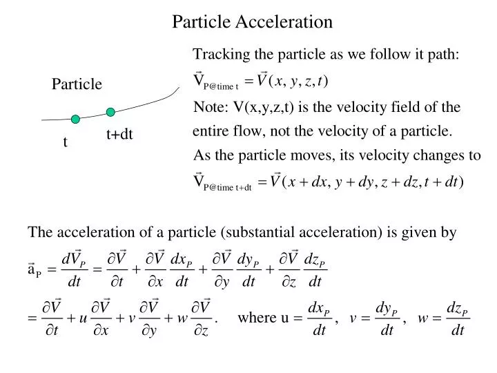
Particle Acceleration. Particle. t+dt. t. Physical Interpretation. Local acceleration. Convective acceleration. Total acceleration of a particle. Unsteady flow. Steady flow. velocity. velocity. acceleration. time. x.

E N D
Particle Acceleration Particle t+dt t
Physical Interpretation Local acceleration Convective acceleration Total acceleration of a particle Unsteady flow Steady flow velocity velocity acceleration time x
An incompressible, inviscid flow past a circular cylinder of diameter d is shown below. The flow variation along the approaching stagnation streamline (A-B) can be expressed as: Example y x A B R=1 m Along A-B streamline, the velocity drops very fast as the particle approaches the cylinder. At the surface of the cylinder, the velocity is zero (stagnation point) and the surface pressure is a maximum. UO=1 m/s
Example (cont.) Determine the acceleration experienced by a particle as it flows along the stagnation streamline. • The particle slows down due to the strong deceleration as it approaches the cylinder. • The maximum deceleration occurs at x=-1.29R=-1.29 m with a magnitude of a(max)=-0.372(m/s2)
Example (cont.) Determine the pressure distribution along the streamline using Bernoulli’s equation. Also determine the stagnation pressure at the stagnation point. • The pressure increases as the particle approaches the stagnation point. • It reaches the maximum value of 0.5, that is Pstag-P=(1/2)rUO2 as u(x)0 near the stagnation point.
Momentum Conservation y x z
Momentum Balance (cont.) Shear stresses (note: tzx: shear stress acting on surfaces perpendicular to the z-axis, not shown in previous slide) Body force Normal stress
Euler’s Equations Note: Integration of the Euler’s equations along a streamline will give rise to the Bernoulli’s equation.
Navier and Stokes Equations For a viscous flow, the relationships between the normal/shear stresses and the rate of deformation (velocity field variation) can be determined by making a simple assumption. That is, the stresses are linearly related to the rate of deformation (Newtonian fluid). (see chapter 5-4.3) The proportional constant for the relation is the dynamic viscosity of the fluid (m). Based on this, Navier and Stokes derived the famous Navier-Stokes equations: