Download
1 / 96
960 likes | 982 Views
Accelerator Physics Particle Acceleration. S. A. Bogacz, G. A. Krafft, S. DeSilva, R. Gamage Old Dominion University Jefferson Lab Lecture 6. RF Acceleration. Characterizing Superconducting RF (SRF) Accelerating Structures Terminology Energy Gain, R/Q , Q 0 , Q L and Q ext

E N D
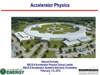
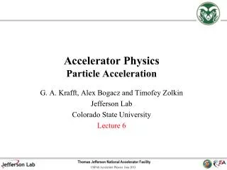
Accelerator PhysicsParticle Acceleration S. A. Bogacz, G. A. Krafft, S. DeSilva, R. Gamage Old Dominion University Jefferson Lab Lecture 6
RF Acceleration • Characterizing Superconducting RF (SRF) Accelerating Structures • Terminology • Energy Gain, R/Q, Q0, QL and Qext • RF Equations and Control • Coupling Ports • Beam Loading • RF Focusing • Betatron Damping and Anti-damping
Terminology 5 Cell Cavity 1 CEBAF Cavity “Cells” 9 Cell Cavity 1 DESY Cavity
Modern Jefferson Lab Cavities (1.497 GHz) are optimized around a 7 cell design Typical cell longitudinal dimension: λRF/2 Phase shift between cells: π Cavities usually have, in addition to the resonant structure in picture: (1) At least 1 input coupler to feed RF into the structure (2) Non-fundamental high order mode (HOM) damping (3) Small output coupler for RF feedback control
Some Fundamental Cavity Parameters • Energy Gain • For standing wave RF fields and velocity of light particles • Normalize by the cavity length L for gradient
Shunt Impedance R/Q • Ratio between the square of the maximum voltage delivered by a cavity and the product of ωRFand the energy stored in a cavity (using “accelerator” definition) • Depends only on the cavity geometry, independent of frequency when uniformly scale structure in 3D • Piel’s rule: R/Q~100 Ω/cell
Unloaded Quality Factor • As is usual in damped harmonic motion define a quality factor by • Unloaded Quality Factor Q0 of a cavity • Quantifies heat flow directly into cavity walls from AC resistance of superconductor, and wall heating from other sources.
Loaded Quality Factor • When add the input coupling port, must account for the energy loss through the port on the oscillation • Coupling Factor • It’s the loaded quality factor that gives the effective resonance width that the RF system, and its controls, seen from the superconducting cavity • Chosen to minimize operating RF power: current matching (CEBAF, FEL), rf control performance and microphonics (SNS, ERLs)
Q0 vs. Gradient for Several 1300 MHz Cavities Courtesey: Lutz Lilje
Eacc vs. time Courtesey: Lutz Lilje
RF Cavity Equations • Introduction • Cavity Fundamental Parameters • RF Cavity as a Parallel LCR Circuit • Coupling of Cavity to an rf Generator • Equivalent Circuit for a Cavity with Beam Loading • On Crest and on Resonance Operation • Off Crest and off Resonance Operation • Optimum Tuning • Optimum Coupling • RF cavity with Beam and Microphonics • Qext Optimization under Beam Loading and Microphonics • RF Modeling
Introduction • Goal: Ability to predict rf cavity’s steady-state response and develop a differential equation for the transient response • We will construct an equivalent circuit and analyze it • We will write the quantities that characterize an rf cavity and relate them to the circuit parameters, for a) a cavity b) a cavity coupled to an rf generator c) a cavity with beam d) include microphonics
RF Cavity Fundamental Quantities • Quality Factor Q0: • Shunt impedance Ra (accelerator definition); • Note: Voltages and currents will be represented as complex quantities, denoted by a tilde. For example: • where is the magnitude of and is a slowly varying phase.
Equivalent Circuit for an rf Cavity Simple LC circuit representing an accelerating resonator. Metamorphosis of the LC circuit into an accelerating cavity. Chain of weakly coupled pillbox cavities representing an accelerating cavity. Chain of coupled pendula as its mechanical analogue.
Equivalent Circuit for an RF Cavity • An rf cavity can be represented by a parallel LCR circuit: • Impedance Z of the equivalent circuit: • Resonant frequency of the circuit: • Stored energy W:
Equivalent Circuit for an RF Cavity • Average power dissipated in resistor R: • From definition of shunt impedance • Quality factor of resonator: • Note: Wiedemann 19.11
Cavity with External Coupling • Consider a cavity connected to an rf source • A coaxial cable carries power from an rf source to the cavity • The strength of the input coupler is adjusted by changing the penetration of the center conductor • There is a fixed output coupler, the transmitted power probe, which picks up power transmitted through the cavity
Cavity with External Coupling Consider the rf cavity after the rf is turned off. Stored energy W satisfies the equation: Total power being lost, Ptot, is: Pe is the power leaking back out the input coupler. Pt is the power coming out the transmitted power coupler. Typically Pt is very small Ptot Pdiss + Pe Recall Energy in the cavity decays exponentially with time constant:
Decay rate equation suggests that we can assign a quality factor to each loss mechanism, such that where, by definition, Typical values for CEBAF 7-cell cavities: Q0=1x10¹⁰, QeQL=2x10⁷.
Have defined “coupling parameter”: and therefore It tells us how strongly the couplers interact with the cavity. Large implies that the power leaking out of the coupler is large compared to the power dissipated in the cavity walls. Wiedemann 19.9
Cavity Coupled to an RF Source • The system we want to model. A generator producing power Pg transmits power to cavity through transmission line with characteristic impedance Z0 • Between the rf generator and the cavity is an isolator – a circulator connected to a load. Circulator ensures that signals reflected from the cavity are terminated in a matched load. Z0 Z0
Transmission Lines … Inductor Impedance and Current Conservation
Transmission Line Equations • Standard Difference Equation with Solution • Continuous Limit ( N → ∞)
Cavity Coupled to an RF Source • Equivalent Circuit RF Generator + Circulator CouplerCavity • Coupling is represented by an ideal (lossless) transformer of turns ratio 1:k
Cavity Coupled to an RF Source • From transmission line equations, forward power from RF source • Reflected power to circulator • Transformer relations • Considering zero forward power case and definition of β
Cavity Coupled to an RF Source • Loaded cavity looks like • Effective and loaded resistance • Solving transmission line equations Wiedemann Fig. 19.1 Wiedemann 19.1
Powers Calculated • Forward Power • Reflected Power • Power delivered to cavity is as it must by energy conservation!
Some Useful Expressions • Total energy W, in terms of cavity parameters • Total impedance
When Cavity is Detuned • Define “Tuning angle” : • Note that: Wiedemann 19.13
Optimal β Without Beam • Optimal coupling: W/Pg maximum or Pdiss = Pg • which implies for Δω = 0, β = 1 • This is the case called “critical” coupling • Reflected power is consistent with energy conservation: • On resonance:
Equivalent Circuit: Cavity with Beam • Beam through the RF cavity is represented by a current generator that interacts with the total impedance (including circulator). • Equivalent circuit: ig the current induced by generator, ib beam current • Differential equation that describes the dynamics of the system:
Cavity with Beam • Kirchoff’s law: • Total current is a superposition of generator current and beam current and beam current opposes the generator current. • Assume that voltages and currents are represented by complex phasors where is the generator angular frequency and are complex quantities.
Voltage for a Cavity with Beam • Steady state solution where is the tuning angle. • Generator current • For short bunches: where I0 is the average beam current. Wiedemann 19.19
Voltage for a Cavity with Beam • At steady-state: are the generator and beam-loading voltages on resonance and are the generator and beam-loading voltages.
Voltage for a Cavity with Beam • Note that: Wiedemann 19.16 Wiedemann 19.20
Voltage for a Cavity with Beam As increases, the magnitudes of both Vg and Vb decrease while their phases rotate by .
Example of a Phasor Diagram Wiedemann Fig. 19.3
On Crest/On Resonance Operation • Typically linacs operate on resonance and on crest in order to receive maximum acceleration. • On crest and on resonance where Vc is the accelerating voltage.
More Useful Equations • We derive expressions for W, Va, Pdiss, Preflin terms of and the loading parameter K, defined by: K=I0Ra/(2 Pg ) From:
Clarifications • On Crest, • Off Crest with Detuning
More Useful Equations • For large, • For Prefl=0 (condition for matching)
Example • For Vc=14 MV, L=0.7 m, QL=2x10⁷ , Q0=1x10¹⁰ :
Off Crest/Off Resonance Operation • Typically electron storage rings operate off crest in order to ensure stability against phase oscillations. • As a consequence, the rf cavities must be detuned off resonance in order to minimize the reflected power and the required generator power. • Longitudinal gymnastics may also impose off crest operation in recirculating linacs. • We write the beam current and the cavity voltage as • The generator power can then be expressed as: Wiedemann 19.30
Off Crest/Off Resonance Operation • Condition for optimum tuning: • Condition for optimum coupling: • Minimum generator power: Wiedemann 19.36
Bettor Phasor Diagram • Off crest, synchrotron phase
C75 Power Estimates G. A. Krafft
12 GeV Project Specs 13 kW Delayen and Krafft TN-07-29 460 µA*15 MV=6.8 kW
Assumptions • Low Loss R/Q = 903*5/7 = 645 Ω • Max Current to be accelerated 460 µA • Compute 0 and 25 Hz detuning power curves • 75 MV/cryomodule (18.75 MV/m) • Therefore matched power is 4.3 kW (Scale increase 7.4 kW tube spec) • Qext adjustable to 3.18×10⁷(if not need more RF power!)