Download
1 / 63
630 likes | 807 Views
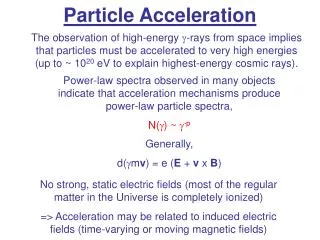
Particle Transport (and a little Particle Acceleration). Gordon Emslie Oklahoma State University. Evidence for Energetic Particles. Particles escaping into interplanetary space Hard X-ray emission (electrons) Gamma-ray emission (electrons and ions) Radio emission (electrons)

E N D
Particle Transport (and a little Particle Acceleration) Gordon Emslie Oklahoma State University
Evidence for Energetic Particles • Particles escaping into interplanetary space • Hard X-ray emission (electrons) • Gamma-ray emission (electrons and ions) • Radio emission (electrons) • Will focus mostly on electrons in this talk
Inversion of Photon Spectra I()= K F(E) (,E) dE (,E) = /E J()= I() = K G(E) dE G(E) = -(1/K) dJ()/d G(E) ~ J()
Key point! Emission process is straightforward, and so it is easy to ascertain the number of electrons from the observed number of photons!
Required Particle Fluxes/Currents/Powers/Energies • (Miller et al. 1997; straightforwardly proportional to observed photon flux) • Electrons • 1037 s-1 > 20 keV • 1018 Amps • 3 1029 ergs s-1 for 100 s = 3 1031 ergs • Ions • 1035 s-1 > 1 MeV • 1016 Amps • 2 1029 ergs s-1 for 100 s = 2 1031 ergs
Electron Number Problem 1037 s-1 > 20 keV Number of electrons in loop = nV ~ 1037 All electrons accelerated in 1 second! Need replenishment of acceleration region!
Electron Current Problem • Steady-state (Ampère): • B = oI/2r ~ (10-6)(1018)/108 = 104 T = 108 G • (B2/8) V ~ 1041 ergs! • Transient (Faraday): • V = (ol) dI/dt = (10-6)(107)(1018)/10 ~ 1018 V!! • So either • (1) currents must be finely filamented; or • (2) particle acceleration is in random directions
An Acceleration Primer F = qEpart; Epart = Elab + vpartB • Epart large-scale coherent acceleration • Epart small-scale stochastic acceleration
Acceleration by Large-Scale Electric Fields m dv/dt = q Epart – m v • Suppose ~ vn-1 dv/dt = (q/m) Epart – vn = a – vn Letvc = a1/n; u = v/vc; = at/vc du/d = 1 – un • For air drag, ~v (n = 2) • For electron in plasma, ~1/v3 (n = -2)
Acceleration Trajectories du/d = 1 - un du/d n<0, unstable 1 u increasing 1 u u decreasing n>0, stable
The Dreicer Field • Recall vc = a1/n~ Epart-1/2 • If vc = vth, Epart = ED – the Dreicer field (ED ~ 10-8 n(cm-3)/T(K) V cm-1 ~ 10-4 V cm-1) vc = vth(E/ED)-1/2 • If E < ED, vc > vth – runaway tail • If E > ED, vc < vth – bulk energization
Sub-Dreicer Acceleration Emergent spectrum is flat! z L-z F=eE dz z=L dn/dt (particles with v > vcrit) E=eE(L-z); dE=eEdz; F(E)dE=(dn/dt)dz →F(E)=(1/eE )(dn/dt)
Accelerated Spectrum F(E ) background Maxwellian runaway tail; height ~ dn/dt eE L E
Computed Runaway Distributions (Sommer 2002, Ph.D. dissertation, UAH)
Accelerated Spectrum • Predicted spectrum is flat • Observed spectrum is ~ power law • Need many concurrent acceleration regions, with range of E and L
Sub-Dreicer Geometry Accelerated particles Accelerated particles “Acceleration Regions” Replenishment Replenishment ~1012 acceleration regions required! Current closure mechanism?
Sub-Dreicer Acceleration • Long (~109 cm) acceleration regions • Weak(< 10-4 V cm-1) fields • Small fraction of particles accelerated • Replenishment and current closure are challenges • Fundamental spectral form is flat • Need large number of current channels to account for observed spectra and to satisfy global electrodynamic constraints
Super-Dreicer Acceleration • Short-extent (~105 cm) strong (~1 V cm-1) fields in large, thin (!) current sheet
Super-Dreicer Acceleration Geometry y Field-aligned acceleration Bx Ez v x Bz By By v Bx Motion out of acceleration region
Super-Dreicer Acceleration • Short (~105 cm) acceleration regions • Strong(> 10V cm-1) fields • Large fraction of particles accelerated • Can accelerate both electrons and ions • Replenishment and current closure are straightforward • No detailed spectral forms available • Need very thin current channels – stability?
(First-order) Fermi Acceleration L v -U U – (v+2U) dv/dt ~ v/t = 2U/(L/v) = (2U/L)v v ~ e(2U/L)t (requires v > U for efficient acceleration!)
Second-order Fermi Acceleration • Energy gain in head-on collisions • Energy loss in “overtaking collisions” BUT number of head-on collisions exceeds number of overtaking collisions → Net energy gain!
Stochastic Fermi Acceleration(Miller, LaRosa, Moore) • Requires the injection of large-scale turbulence and subsequent cascade to lower sizescales • Large-amplitude plasma waves, or magnetic “blobs”, distributed throughout the loop • Adiabatic collisions with converging scattering centers give 2nd-order Fermi acceleration (as long as v > U! )
Stochastic Fermi Acceleration • Thermal electrons have v>vA and are efficiently accelerated immediately • Thermal ions take some time to reach vA and hence take time to become efficiently accelerated
Stochastic Acceleration t = 0 – 0.1 s
Stochastic Acceleration • Accelerates both electrons and ions • Electrons accelerated immediately • Ions accelerated after delay, and only in long acceleration regions • Fundamental spectral forms are power-laws
Electron vs. Ion Acceleration and Transport • If ion and electron acceleration are produced by the same fundamental process, then the gamma-rays produced by the ions should be produced in approximately the same location as the hard X-rays produced by the electrons
Observations: 2002 July 23 Flare Ion acceleration favored on longer loops!
Particle Transport Cross-section dE/dt = n v E cm-3 erg s-1 erg cm s-1 cm2
Coulomb collisions • = 2e4Λ/E2; • Λ = “Coulomb logarithm” ~ 20) • dE/dt = -(2e4Λ/E) nv = -(K/E) nv • dE/dN = -K/E; dE2/dN = -2K • E2 = Eo2 – 2KN
Spectrum vs. Depth • Continuity: F(E) dE = Fo(Eo)dEo • Transport: E2 = Eo2 – 2KN; E dE = Eo dEo • F(E) = Fo(Eo) dEo/dE = (E/Eo) Fo(Eo) • F(E) = (E/ ([E2 + 2KN]1/2)Fo([E2 + 2KN]1/2)
Spectrum vs. Depth F(E) = (E/ ([E2 + 2KN]1/2)Fo([E2 + 2KN]1/2) (a) 2KN << E2 F(E) ~ Fo(E) (b) 2KN >> E2 F(E) ~ (E/[2KN]1/2) Fo([2KN]1/2) ~ E Also, v f(v) dv = F(E) dE f(v) = m F(E)
Spectrum vs. Depth Resulting photon spectrum gets harder with depth!
Return Current • dE/ds = -eE, E = electric field • Ohm’s Law: E = η j = ηeF, F = particle flux • dE/ds = -ηe2F • dE/ds independent of E: E = Eo – e2 ∫ ηF ds • note that F = F[s] due to transport and η = η(T)
Return Current • Zharkova results
Return Current • dE/ds = -ηe2F • Penetration depth s ~ 1/F • Bremsstrahlung emitted ~ F (1/F) – independent of F! • Saturated flux limit – very close to observed value!
Magnetic Mirroring • F = - dB/ds; = magnetic moment • Does not change energy, but causes redirection of momentum • Indirectly affects energy loss due to other processes, e.g. • increase in pitch angle reduces flux F and so electric field strength E • Penetration depth due to collisions changed.
Temporal Trends N M S
Implications for Particle Transport • Spectrum at one footpoint (South) consistently harder • This is consistent with collisional transport through a greater mass of material!
Atmospheric Response • Collisional heating temperature rise • Temperature rise pressure increase • Pressure increase mass motion • Mass motion density changes • “Evaporation”