Download
1 / 20
200 likes | 405 Views
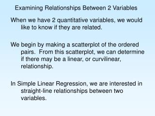
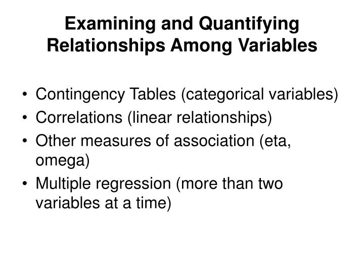
Examining and Quantifying Relationships Among Variables. Contingency Tables (categorical variables) Correlations (linear relationships) Other measures of association (eta, omega) Multiple regression (more than two variables at a time). Contingency Tables

E N D
Examining and Quantifying Relationships Among Variables • Contingency Tables (categorical variables) • Correlations (linear relationships) • Other measures of association (eta, omega) • Multiple regression (more than two variables at a time)
Contingency Tables When all of your variables are categorical, you can use contingency tables to see if your variables are related. • A contingency table is a table displaying information in cells formed by the intersection of two or more categorical variables. • A contingency or relationship occurs when there is a pattern between the data on the rows with the data on the columns
Relationship Between Size of Hospital and Length of Stay in Hospital Phi = .405
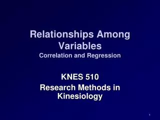
Examining and Quantifying Relationships Among Variables • Measures of association • Correlation coefficient, r • Other strength of association measures, eta (η), omega (ω) • Percentage of Variance Explained (PVE): (association measure)2 X 100 • For example, r = .7, PVE = (.7)2 X 100 = 49%
Pearson’s correlation coefficient • Correlation – measure of the linear relationship between two variables • Coefficient can range from 0 to +/- 1.00 • Size of number indicates strength or magnitude of relationship • Sign indicates direction of relationship
Four sets of data with the same correlation of 0.81, as described by F. Anscombe.
Illustration of Strength of Relationship Using Venn-like Diagrams Y X r2 = 0.0 X Y X Y r2 = 0.30 r2 = 0.95
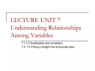
Correlation vs. Regression • Correlation investigates relationships between variables • Variables have equal status or role • Regression examines relationship of predictor variable(s) on outcome variable • Variables have different role or status, interest of researcher is directional • Predictor variables (X’s) predict or explain the outcome variable (Y)
Correlation, bidirectional Regression, X influences Y, unidirectional
Regression Analysis • Regression analysis: used to explain or predict the values of a quantitative dependent variable based on the values of one or more predictor variables. • • Simple regression, one predictor variable. • • Multiple regression, two or more predictor variables. • Here is the simple regression equation showing the relationship between starting salary (Y or your dependent variable) and GPA (X or your independent variable): • Y = 9,234.56 + 7,638.85 (X)
• The 9,234.56 is the Y intercept (look at the above regression line; it crosses the Y axis a little below $10,000; specifically, it crosses the Y axis at $9,234.56). • The 7,638.85 is the simple regression coefficient, which tells you the average amount of increase in starting salary that occurs when GPA increases by one unit. (It is also the slope or the rise over the run). • Now, you can plug in a value for X (i.e., starting salary) and easily get the predicted starting salary. • If you put in a 3.00 for GPA in the above equation and solve it, you will see that the predicted starting salary is $32,151.11 • Now plug in another number within the range of the data (how about a 3.5) and see what the predicted starting salary is. (Check on your work: it is $35,970.54)
Multiple Regression: examining more than one association at the same time • • Main difference between simple and multiple regression is that multiple looks at the complex relationships among several predictors at the same time. The regression coefficient is now called a partial regression coefficient. This coefficient provides the predicted change in the dependent variable given a one unit change in the predictor variable, controlling for the other predictor variables in the equation. In other words, you can use multiple regression to control for other variables (i.e., statistical control). • Kinds of coefficients • Raw score betas (unique relationship controlling for other predictors) • Standardized betas (unique relationship controlling for other predictors) • R and R2(all predictors together) • Multicollinearity
Shared Variance in Multiple Regression, all overlap = R2
Unique overlap of an individual predictor (x2) is standardized beta All overlap of an individual predictor (x2) is Pearson’s r2
Y X2 X1 Multicollinearity is the area the two predictors have in common, the extent to which the two predictors correlate with each other