Download
1 / 37
370 likes | 522 Views
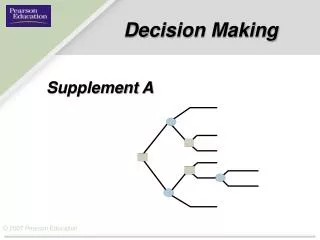
Decision Making. Supplement A. Objectives. Apply break-even analysis, using both the graphic and algebraic approaches, to evaluate new products and services and different process methods. evaluate decision alternatives with a preference matrix for multiple criteria.

E N D
Decision Making Supplement A
Objectives • Apply break-even analysis, using both the graphic and algebraic approaches, to evaluate new products and services and different process methods. • evaluate decision alternatives with a preference matrix for multiple criteria. • Construct a payoff table and then select the best alternative by using a decision rule such as maximin, maximax, Laplace, minimax regret, or expected value. • Calculate the value of perfect information. • Draw and analyze a decision tree.
Quantity Total Annual Total Annual (patients) Cost ($) Revenue ($) (Q) (100,000 + 100Q) (200Q) 0 100,000 0 2000 300,000 400,000 Break-Even Analysis Total Cost = Fixed Cost + Variable Cost * Volume sold Total Revenue = Revenue per unit * Volume Sold Revenue = Cost = pQ = F + cQ Break Even Point = Fixed Cost / (revenue – variable cost)
Quantity Total Annual Total Annual (patients) Cost ($) Revenue ($) (Q) (100,000 + 100Q) (200Q) (2000, 400) 0 100,000 0 2000 300,000 400,000 Total annual revenues Dollars (in thousands) | | | | 500 1000 1500 2000 Patients (Q) Break-Even Analysis 400 – 300 – 200 – 100 – 0 –
Break-Even Analysis 400 – 300 – 200 – 100 – 0 – (2000, 400) (2000, 300) Total annual revenues Total annual costs Dollars (in thousands) (0, 100) Fixed costs (0, 0) | | | | 500 1000 1500 2000 Patients (Q)
400 – 300 – 200 – 100 – 0 – (2000, 400) Profits (2000, 300) Total annual revenues Total annual costs Dollars (in thousands) Break-even quantity Fixed costs Loss | | | | 500 1000 1500 2000 Patients (Q) Break-Even Analysis
400 – 300 – 200 – 100 – 0 – Profits Total annual revenues Total annual costs Dollars (in thousands) Forecast = 1,500 Fixed costs Loss | | | | 500 1000 1500 2000 Example A.2 Patients (Q) Sensitivity Analysis
pQ – (F + cQ) 200(1500) – [100,000 + 100(1500)] = $50,000 Profits Total annual revenues Total annual costs Dollars (in thousands) Forecast = 1,500 Fixed costs Loss | | | | 500 1000 1500 2000 Patients (Q) Sensitivity Analysis 400 – 300 – 200 – 100 – 0 –
Threshold score = 800 Performance Weight Score Weighted Score Criterion (A) (B) (A x B) Market potential 30 8 240 Unit profit margin 20 10 200 Operations compatibility 20 6 120 Competitive advantage 15 10 150 Investment requirement 10 2 20 Project risk 5 4 20 Weighted score = 750 Preference Matrix Example A.4
Threshold score = 800 Performance Weight Score Weighted Score Criterion (A) (B) (A x B) Market potential 30 8 240 Unit profit margin 20 10 200 Operations compatibility 20 6 120 Competitive advantage 15 10 150 Investment requirement 10 2 20 Project risk 5 4 20 Weighted score = 750 Not At This Time Example A.4 Preference Matrix
Possible Future Demand Alternative Low High Small facility 200 270 Large facility 160 800 Do nothing 0 0 If future demand will be low—Choose the small facility. Decision Theory: Under Certainty Example A.5
Possible Future Demand Alternative Low High Small facility 200 270 Large facility 160 800 Do nothing 0 0 Under Uncertainty Example A.6
Possible Future Demand Maximin—Small Alternative Low High Small facility 200 270 Large facility 160 800 Do nothing 0 0 Best of the worst Under Uncertainty Example A.6
Possible Future Demand Maximin—Small Maximax—Large Alternative Low High Small facility 200 270 Large facility 160 800 Do nothing 0 0 Best of the best Under Uncertainty Example A.6
Possible Future Demand Maximin—Small Maximax—Large Laplace—Large Alternative Low High Small facility 200 270 Large facility 160 800 Do nothing 0 0 Best weighted payoff Small facility 0.5(200) + 0.5(270) = 235 Large facility 0.5(160) + 0.5(800) = 480 Example A.6 Under Uncertainty
Possible Future Demand Maximin—Small Maximax—Large Laplace—Large Minimax Regret—Large Alternative Low High Small facility 200 270 Large facility 160 800 Do nothing 0 0 Regret Low Demand High Demand Small facility 200 – 200 = 0 800 – 270 = 530 Large facility 200 – 160 = 40 800 – 800 = 0 Best worst regret Example A.6 Under Uncertainty
Possible Future Demand Maximin—Small Maximax—Large Laplace—Large Minimax Regret—Large Alternative Low High Small facility 200 270 Large facility 160 800 Do nothing 0 0 Under Uncertainty Example A.6
Possible Future Demand Psmall = 0.4 Plarge = 0.6 Alternative Low High Small facility 200 270 Large facility 160 800 Do nothing 0 0 Alternative Expected Value Small facility 0.4(200) + 0.6(270) = 242 Large facility 0.4(160) + 0.6(800) = 544 Example A.7 Under Risk
Possible Future Demand Psmall = 0.4 Plarge = 0.6 Alternative Low High Small facility 200 270 Large facility 160 800 Do nothing 0 0 Alternative Expected Value Small facility 0.4(200) + 0.6(270) = 242 Large facility 0.4(160) + 0.6(800) = 544 Example A.7 Under Risk Highest Expected Value
Under Risk Figure A.4
Possible Future Demand Psmall = 0.4 Plarge = 0.6 Alternative Low High Small facility 200 270 Large facility 160 800 Do nothing 0 0 Event Best Payoff Low demand 200 High demand 800 Example A.8 Perfect Information
Possible Future Demand Psmall = 0.4 Plarge = 0.6 Alternative Low High Small facility 200 270 Large facility 160 800 Do nothing 0 0 Event Best Payoff Low demand 200 EVperfect = 200(0.4) + 800(0.6) = 560 High demand 800 EVimperfect = 160(0.4) + 800(0.6) = 544 Example A.8 Perfect Information
Possible Future Demand Psmall = 0.4 Plarge = 0.6 Alternative Low High Small facility 200 270 Large facility 160 800 Do nothing 0 0 Event Best Payoff Low demand 200 EVperfect = 200(0.4) + 800(0.6) = 560 High demand 800 EVimperfect = 160(0.4) + 800(0.6) = 544 Value of perfect information = $560,000 - $544,000 Example A.8 Perfect Information
E1 [P(E1)] E2 [P(E2)] E3 [P(E3)] Payoff 1 Payoff 2 Payoff 3 Alternative 1 Alternative 3 Alternative 4 Alternative 5 Payoff 1 Payoff 2 Payoff 3 1 2 1st decision Possible 2nd decision E1 [P(E1)] Alternative 2 E2 [P(E2)] E3 [P(E3)] Payoff 1 Payoff 2 = Event node = Decision node Ei = Event i Figure A.5 P(Ei) = Probability of event i Decision Trees
Low demand [0.4] $200 $223 $270 $40 $800 Don’t expand Expand Do nothing Advertise High demand [0.6] Small facility 2 1 Modest response [0.3] Sizable response [0.7] $20 $220 3 Large facility Low demand [0.4] High demand [0.6] Example A.9 Decision Trees
Low demand [0.4] $200 $223 $270 $40 $800 Don’t expand Expand Do nothing Advertise High demand [0.6] Small facility 2 0.3(20) + 0.7(220) 1 Modest response [0.3] Sizable response [0.7] $20 $220 3 Large facility Low demand [0.4] High demand [0.6] Example A.9 Decision Trees
Low demand [0.4] $200 $223 $270 $40 $800 Don’t expand Expand Do nothing Advertise High demand [0.6] Small facility 2 0.3(20) + 0.7(220) 1 Modest response [0.3] Sizable response [0.7] $20 $220 3 Large facility Low demand [0.4] $160 High demand [0.6] Example A.9 Decision Trees
Low demand [0.4] $200 $223 $270 $40 $800 Don’t expand Expand Do nothing Advertise High demand [0.6] Small facility 2 $270 1 Modest response [0.3] Sizable response [0.7] $20 $220 3 Large facility Low demand [0.4] $160 $160 High demand [0.6] Example A.9 Decision Trees
Low demand [0.4] $200 $223 $270 $40 $800 0.4(200) + 0.6(270) Don’t expand Expand Do nothing Advertise High demand [0.6] Small facility 2 $270 1 Modest response [0.3] Sizable response [0.7] $20 $220 3 Large facility Low demand [0.4] $160 0.4(160) + 0.6(800) ($160) High demand [0.6] Example A.9 Decision Trees
Low demand [0.4] $200 $223 $270 $40 $800 0.4(200) + 0.6(270) Don’t expand Expand Do nothing Advertise High demand [0.6] $242 Small facility 2 $270 1 Modest response [0.3] Sizable response [0.7] $20 $220 3 Large facility Low demand [0.4] $160 0.4(160) + 0.6(800) ($160) $544 High demand [0.6] Example A.9 Decision Trees
Low demand [0.4] $200 $223 $270 $40 $800 Don’t expand Expand Do nothing Advertise High demand [0.6] $242 Small facility 2 $270 1 $544 Modest response [0.3] Sizable response [0.7] $20 $220 3 Large facility Low demand [0.4] $160 $160 $544 High demand [0.6] Decision Trees Example A.9
250 – 200 – 150 – 100 – 50 – 0 – Total revenues Break-even quantity Dollars (in thousands) $77.7 Total costs 3.1 | | | | | | | | 1 2 3 4 5 6 7 8 Units (in thousands) Solved Problem 1 BE Revenue = pQ Revenue = 25*3111 Revenue = $77,775
Solved Problem 3 • To determine the payoff amounts: Buy roses for $15 dozen Sell roses for $40 dozen Sell 25, Order 25, = pQ – cQ = 40(25) – 15(25) =625 Sell 60,Order 130 = pQ – cQ = 40(60) – 15(130) = 450
Solved Problem 3 • Maximin – best of the worst. If demand is Low, the best alternative is to order 25 dozen. • Maximax – best of the best. If demand is high, the best alternative is to order 130 dozen. • Laplace – Best weighted payoff. • 25 dozen: 625(.33) + 625(.33) +625(.33) = 625 • 60 dozen: 100(.33) + 1500(.33) + 1500(.33) = 1023 • 130 dozen: -950(.33) + 450(.33) + 3250(.33) = 907
Solved Problem 3 Best Payoff: 625 1500 3250
Solved Problem • Minimax Regret –best “worst regret” • Maximum regret of 25 dozen occurs if demand is high: $3250 – $625 = $2625 • Maximum regret of 60 dozen occurs if demand is high: $3250 - $1500 = $1750 • Maximum regret of 130 dozen occurs if demand is low: $625 - -$950 = $1575 • The minimum of regrets is ordering 130 dozen!
Bad times [0.3] Bad times [0.3] $191 Normal times [0.5] Normal times [0.5] $240 One lift $225.3 Good times [0.2] Good times [0.2] $240 $256.0 $151 Two lifts $245 $256.0 $441 Figure A.8 Solved Problem 4