Download
1 / 56
610 likes | 817 Views
Decision Making. Supplement A. Break-Even Analysis. Break-even analysis is used to compare processes by finding the volume at which two different processes have equal total costs. Break-even point is the volume at which total revenues equal total costs.

E N D
Decision Making Supplement A
Break-Even Analysis • Break-even analysis is used to compare processes by finding the volume at which two different processes have equal total costs. • Break-even point is the volume at which total revenues equal total costs. • Variable costs (c) are costs that vary directly with the volume of output. • Fixed costs (F) are those costs that remain constant with changes in output level.
Break-Even Analysis • “Q” is the volume of customers or units, “c” is the unit variable cost, F is fixed costs and p is the revenue per unit • cQ is the total variable cost. • Total cost =F + cQ • Total revenue =pQ • Break-even is wherepQ = F + cQ(Total revenue = Total cost)
Break-Even Analysis can tell you… • If a forecast sales volume is sufficient to break even (no profit or no loss) • How low variable cost per unit must be to break even given current prices and sales forecast. • How low the fixed cost need to be to break even. • How price levels affect the break-even volume.
Hospital ExampleExample A.1 A hospital is considering a new procedure to be offered at $200 per patient. The fixed cost per year would be $100,000, with total variable costs of $100 per patient. What is the break-even quantity for this service? = 1,000 patients Q = F / (p - c) = 100,000 / (200-100)
Quantity Total Annual Total Annual (patients) Cost ($) Revenue ($) (Q) (100,000 + 100Q) (200Q) 0 100,000 0 2000 300,000 400,000 Dollars (in thousands) | | | | 500 1000 1500 2000 Patients (Q) 400 – 300 – 200 – 100 – 0 – Hospital ExampleExample A.1continued
Quantity Total Annual Total Annual (patients) Cost ($) Revenue ($) (Q) (100,000 + 100Q) (200Q) Quantity Total Annual Total Annual (patients) Cost ($) Revenue ($) (Q) (100,000 + 100Q) (200Q) (2000, 400) 0 100,000 0 2000 300,000 400,000 0 100,000 0 2000 300,000 400,000 Dollars (in thousands) | | | | 500 1000 1500 2000 Patients (Q) 400 – 300 – 200 – 100 – 0 – Total annual revenues
Quantity Total AnnualTotal Annual (patients) Cost ($)Revenue ($) (Q) (100,000 + 100Q)(200Q) 400 – 300 – 200 – 100 – 0 – (2000, 400) 0 100,0000 2000 300,000400,000 (2000, 300) Total annual costs Dollars (in thousands) Fixed costs | | | | 500 1000 1500 2000 Patients (Q) Total annual revenues
Quantity Total AnnualTotal Annual (patients) Cost ($)Revenue ($) (Q) (100,000 + 100Q)(200Q) 400 – 300 – 200 – 100 – 0 – (2000, 400) 0 100,0000 2000 300,000400,000 Profits Total annual revenues (2000, 300) Total annual costs Dollars (in thousands) Break-even quantity Fixed costs Loss | | | | 500 1000 1500 2000 Patients (Q)
400 – 300 – 200 – 100 – 0 – pQ – (F + cQ) 200(1500) – [100,000 + 100(1500)] $50,000 Profits Total annual revenues Total annual costs Dollars (in thousands) Forecast = 1,500 Fixed costs Loss | | | | 500 1000 1500 2000 Patients (Q) Sensitivity AnalysisExample A.2
Application A.1Solution Q TR = pQ TC = F + cQ
Application A.1Solution Q TR = pQ TC = F + cQ
Application A.1Solution pQ = F + cQ Q TR = pQ TC = F + pQ
Two Processes and Make-or-Buy Decisions • Breakeven analysis can be used to choose between two processes or between an internal process and buying those services or materials. • The solution finds the point at which the total costs of each of the two alternatives are equal. • The forecast volume is then applied to see which alternative has the lowest cost for that volume.
Breakeven for Two Processes Example A.3
Fm – Fb cb – cm Q = 12,000 – 2,400 2.0 – 1.5 Q = Breakeven forTwo Processes Example A.3
Fm – Fb cb – cm Q = Q = 19,200 salads Breakeven for Two Processes Example A.3
Application A.2 Fm – Fb cb – cm $300,000 – $0$9 – $7 = $150,000 Q = =
Preference Matrix • A Preference Matrix is a table that allows you to rate an alternative according to several performance criteria. • The criteria can be scored on any scale as long as the same scale is applied to all the alternatives being compared. • Each score is weighted according to its perceived importance, with the total weights typically equaling 100. • The total score is the sum of the weighted scores (weight × score) for all the criteria. The manager can compare the scores for alternatives against one another or against a predetermined threshold.
Threshold score = 800 Performance Weight Score Weighted Score Criterion (A) (B) (A x B) Market potential Unit profit margin Operations compatibility Competitive advantage Investment requirement Project risk Preference MatrixExample A.4
Threshold score = 800 Performance Weight Score Weighted Score Criterion (A) (B) (A x B) Market potential 30 Unit profit margin 20 Operations compatibility 20 Competitive advantage 15 Investment requirement 10 Project risk 5 Preference MatrixExample A.4continued
Threshold score = 800 Performance Weight Score Weighted Score Criterion (A) (B) (A x B) Market potential 30 8 Unit profit margin 20 10 Operations compatibility 20 6 Competitive advantage 15 10 Investment requirement 10 2 Project risk 5 4 Preference MatrixExample A.4continued
Threshold score = 800 Performance Weight Score Weighted Score Criterion (A) (B) (A x B) Market potential 30 8 240 Unit profit margin 20 10 200 Operations compatibility 20 6 120 Competitive advantage 15 10 150 Investment requirement 10 2 20 Project risk 5 4 20 Preference MatrixExample A.4continued
Threshold score = 800 Performance Weight Score Weighted Score Criterion (A) (B) (A x B) Market potential 30 8 240 Unit profit margin 20 10 200 Operations compatibility 20 6 120 Competitive advantage 15 10 150 Investment requirement 10 2 20 Project risk 5 4 20 Weighted score = 750 Preference MatrixExample A.4continued
Threshold score = 800 Performance Weight Score Weighted Score Criterion (A) (B) (A x B) Market potential 30 8 240 Unit profit margin 20 10 200 Operations compatibility 20 6 120 Competitive advantage 15 10 150 Investment requirement 10 2 20 Project risk 5 4 20 Weighted score = 750 Preference MatrixExample A.4continued Score does not meet the threshold and is rejected.
Application A.3 The concept of a weighted score Repeat this process for each alternative — pick the one with the largest weighted score
Decision Theory • Decision theory is a general approach to decision making when the outcomes associated with alternatives are often in doubt. • A manager makes choices using the following process: • List the feasible alternatives • List the chance events (states of nature). • Calculate the payoff for each alternative in each event. • Estimate the probability of each event. (The total probabilities must add up to 1.) • Select the decision rule to evaluate the alternatives.
Decision Rules • Decision Making Under Uncertainty is when you are unable to estimate the probabilities of events. • Maximin: The best of the worst. A pessimistic approach. • Maximax: The best of the best. An optimistic approach. • MinimaxRegret: Minimizing your regret (also pessimistic) • Laplace: The alternative with the best weighted payoff using assumed probabilities. • Decision Making Under Riskis when one is able to estimate the probabilities of the events. • ExpectedValue: The alternative with the highest weighted payoff using predicted probabilities.
Events(Uncertain Demand) Alternatives Low High Small facility 200 270 Large facility 160 800 Do nothing 0 0 MaxiMin DecisionExample A.6 a. Look at the payoffs for each alternative and identify the lowest payoff for each. Choose the alternative that has the highest of these. (the maximum of the minimums)
Events(Uncertain Demand) Alternatives Low High Small facility 200 270 Large facility 160 800 Do nothing 0 0 MaxiMax DecisionExample A.6 b. Look at the payoffs for each alternative and identify the “highest” payoff for each. Choose the alternative that has the highest of these. (the maximum of the maximums)
Events Alternatives Low High (0.5) (0.5) Small facility 200 270 Large facility 160 800 Do nothing 0 0 200*0.5 + 270*0.5 = 235160*0.5 + 800*0.5 = 480 Laplace(Assumed equal probabilities)Example A.6 c. Multiply each payoff by the probability of occurrence of its associated event. Select the alternative with the highest weighted payoff.
Events(Uncertain Demand) Alternatives Low High Small facility 200 270 Large facility 160 800 Do nothing 0 0 MiniMax RegretExample A.6 d. Look at each payoff and ask yourself, “If I end up here, do I have any regrets?” Your regret, if any, is the difference between that payoff and what you could have had by choosing a different alternative, given the same state of nature (event).
Events(Uncertain Demand) Alternatives Low High Small facility 200 270 Large facility 160 800 Do nothing 0 0 If you chose a large facility and demand is low, you have a regret of 40. (The difference between the 160 you got and the 200 you could have had.) If you chose a small facility and demand is low, you have zero regret. MiniMax RegretExample A.6 d. continued
Events(Uncertain Demand) Alternatives Low High Small facility 200 270 Large facility 160 800 Do nothing 0 0 Regret Matrix Events Alternatives Low High Small facility 0 530 Large facility 40 0 Do nothing 200 800 MaxRegret 530 40 800 MiniMax RegretExample A.6 d. continued Building a large facility offers the least regret.
Events Alternatives Low High (0.4) (0.6) Small facility 200 270 Large facility 160 800 Do nothing 0 0 200*0.4 + 270*0.6 = 242160*0.4 + 800*0.6 = 544 Expected ValueDecision Making under RiskExample A.7 Multiply each payoff by the probability of occurrence of its associated event. Select the alternative with the highest weighted payoff.
Expected Value Analysis Example A.7
Application A.4 What is the minimax regret solution? 840 – 840 = 0 710 1150 – 440 = 710 670 – 190 = 480 840 – 370 = 470 1150 – 220 = 930 670 – 670 = 0 930 830 670 – (-25) = 695 840 – 25 = 830 1150 – 1150 = 0
Decision Trees • Decision Treesare schematic models of alternatives available along with their possible consequences. • They are used in sequential decision situations. • Decision points are represented by squares. • Event points are represented by circles.
E1 & Probability E2& Probability E3& Probability Payoff 1 Payoff 2 Payoff 3 Alternative 3 Alternative 4 Alternative 5 Payoff 1 Payoff 2 Payoff 3 Alternative 1 1 2 1st decision Possible 2nd decision E1& Probability Alternative 2 Payoff 1 Payoff 2 E2& Probability E3& Probability Decision Trees = Event node = Decision node
Decision Trees • After drawing a decision tree, we solve it by working from right to left, starting with decisions farthest to the right, and calculating the expected payoff for each of its possible paths. • We pick the alternative for that decision that has the best expected payoff. • We “saw off,” or “prune,” the branches not chosen by marking two short lines through them. • The decision node’s expected payoff is the one associated with the single remaining branch.
Small facility 1 Large facility Drawing the TreeExample A.8
Low demand [0.4] $200 $223 $270 Don’t expand Expand High demand [0.6] Small facility 2 1 Large facility Drawing the TreeExample A.8continued
Low demand [0.4] $200 $223 $270 $40 $800 Don’t expand Expand Do nothing Advertise High demand [0.6] Small facility 2 1 Modest response [0.3] Sizable response [0.7] $20 $220 3 Large facility Low demand [0.4] High demand [0.6] Completed DrawingExample A.8
Low demand [0.4] $200 $223 $270 $40 $800 Don’t expand Expand Do nothing Advertise High demand [0.6] Small facility 2 1 Modest response [0.3] Sizable response [0.7] $20 $220 3 Large facility Low demand [0.4] High demand [0.6] Solving Decision #3Example A.8 0.3 x $20 = $6 $6 + $154 = $160 0.7 x $220 = $154
Low demand [0.4] $200 $223 $270 $40 $800 Don’t expand Expand Do nothing Advertise High demand [0.6] Small facility 2 1 Modest response [0.3] Sizable response [0.7] $20 $220 3 Large facility Low demand [0.4] $160 $160 High demand [0.6] Solving Decision #3Example A.8
Low demand [0.4] $200 $223 $270 $40 $800 Don’t expand Expand Do nothing Advertise High demand [0.6] Small facility 2 $270 1 3 Large facility Low demand [0.4] $160 $160 High demand [0.6] Solving Decision #2Example A.8 Expanding has a higher value. Modest response [0.3] Sizable response [0.7] $20 $220