Download
1 / 67
750 likes | 1.11k Views
A. Decision Making. Break-Even Analysis. Evaluating Services or Products Is the predicted sales volume of the service or product sufficient to break even (neither earning a profit nor sustaining a loss)?

E N D
A Decision Making
Break-Even Analysis • Evaluating Services or Products • Is the predicted sales volume of the service or product sufficient to break even (neither earning a profit nor sustaining a loss)? • How low must the variable cost per unit be to break even, based on current prices and sales forecasts? • How low must the fixed cost be to break even? • How do price levels affect the break-even quantity?
Break-Even Analysis • Break-even analysis is based on the assumption that all costs related to the production of a specific service or product can be divided into two categories: variable costs and fixed costs • Variable cost, c, is the portion of the total cost that varies directly with volume of output • If Q = the number of customers served or units produced per year, total variable cost = cQ • Fixed cost, F, is the portion of the total cost that remains constant regardless of changes in levels of output
F p - c Q = Break-Even Analysis • By setting revenue equal to total cost • So Total cost = F + cQ Total revenue = pQ pQ = F + cQ
100,000 200 – 100 = F p - c Q = Finding the Break-Even Quantity EXAMPLE A.1 A hospital is considering a new procedure to be offered at $200 per patient. The fixed cost per year would be $100,000, with total variable costs of $100 per patient. What is the break-even quantity for this service? Use both algebraic and graphic approaches to get the answer. SOLUTION The formula for the break-even quantity yields = 1,000 patients
Finding the Break-Even Quantity • To solve graphically we plot two lines: one for costs and one for revenues • Begin by calculating costs and revenues for two different output levels • The following table shows the results for Q = 0 and Q = 2,000 • Draw the cost line through points (0, 100,000) and (2,000, 300,000) • Draw the revenue line through (0, 0) and (2,000, 400,000)
400 – 300 – 200 – 100 – 0 – (2000, 400) Total annual revenues (2000, 300) Dollars (in thousands) Fixed costs | | | | 500 1000 1500 2000 Patients (Q) Finding the Break-Even Quantity Profits Total annual costs • The two lines intersect at 1,000 patients, the break-even quantity Break-even quantity Loss FIGURE A.1 – Graphic Approach to Break-Even Analysis
Application A.1 The Denver Zoo must decide whether to move twin polar bears to Sea World or build a special exhibit for them and the zoo. The expected increase in attendance is 200,000 patrons. The data are: Revenues per Patron for Exhibit Gate receipts $4 Concessions $5 Licensed apparel $15 Estimated Fixed Costs Exhibit construction $2,400,000 Salaries $220,000 Food $30,000 Estimated Variable Costs per Person Concessions $2 Licensed apparel $9 • Is the predicted increase in attendance sufficient to break even?
7 – 6 – 5 – 4 – 3 – 2 – 1 – 0 – Total Cost Cost and revenue (millions of dollars) Total Revenue | | | | | | 50 100 150 200 250 Q (thousands of patrons) Application A.1 Where p = 4 + 5 + 15 = $24 F = 2,400,000 + 220,000 + 30,000 = $2,650,000 c = 2 + 9 = $11
Application A.1 Where p = 4 + 5 + 15 = $24 F = 2,400,000 + 220,000 + 30,000 = $2,650,000 c = 2 + 9 = $11 Algebraic solution of Denver Zoo problem pQ = F + cQ 24Q = 2,650,000 + 11Q 13Q = 2,650,000 Q = 203,846
Sensitivity Analysis EXAMPLE A.2 If the most pessimistic sales forecast for the proposed service in Figure A.1 were 1,500 patients, what would be the procedure’s total contribution to profit and overhead per year? SOLUTION The graph shows that even the pessimistic forecast lies above the break-even volume, which is encouraging. The product’s total contribution, found by subtracting total costs from total revenues, is pQ– (F + cQ) = 200(1,500) – [100,000 + 100(1,500)] = $50,000
Evaluating Processes • Choices must be made between two processes or between an internal process and buying services or materials on the outside • We assume that the decision does not affect revenues • The analyst finds the quantity for which the total costs for two alternatives are equal
Fm – Fb cb – cm Q = Evaluating Processes • Let Fb equal the fixed cost (per year) of the buy option, Fm equal the fixed cost of the make option, cb equal the variable cost (per unit) of the buy option, and cm equal the variable cost of the make option • The total cost to buy isFb + cbQ and the total cost to make is Fm + cmQ • To find the break-even quantity, we set the two cost functions equal and solve for Q: Fb+ cbQ= Fm+ cmQ
Break-Even Analysis for Make-or-Buy Decisions • A fast-food restaurant featuring hamburgers is adding salads to the menu • The price to the customer will be the same • Fixed costs are estimated at $12,000 and variable costs totaling $1.50 per salad • Preassembled salads could be purchased from a local supplier at $2.00 per salad • Preassembled salads would require additional refrigeration with an annual fixed cost of $2,400 • Expected demand is 25,000 salads per year • What is the break-even quantity? EXAMPLE A.3
Fm – Fb cb – cm Q = = 12,000 – 2,400 2.0 – 1.5 Break-Even Analysis for Make-or-Buy Decisions SOLUTION The formula for the break-even quantity yields the following: = 19,200 salads Figure A.2 shows the solution from OM Explorer’s Break-Even Analysis Solver. The break-even quantity is 19,200 salads. As the 25,000-salad sales forecast exceeds this amount, the make option is preferred. Only if the restaurant expected to sell fewer than 19,200 salads would the buy option be better.
Break-Even Analysis for Make-or-Buy Decisions FIGURE A.2 – Break-Even Analysis Solver of OM Explorer for Example A.3
$300,000 – $0 $9 – $7 Fm – Fbcb – cm Q = = Application A.2 At what volume should the Denver Zoo be indifferent between buying special sweatshirts from a supplier or have zoo employees make them? = 150,000
Preference Matrix • A Preference Matrix is a table that allows you to rate an alternative according to several performance criteria • The criteria can be scored on any scale as long as the same scale is applied to all the alternatives being compared • Each score is weighted according to its perceived importance, with the total weights typically equaling 100 • The total score is the sum of the weighted scores (weight × score) for all the criteria and compared against scores for alternatives
Evaluating an Alternative EXAMPLE A.4 The following table shows the performance criteria, weights, and scores (1 = worst, 10 = best) for a new thermal storage air conditioner. If management wants to introduce just one new product and the highest total score of any of the other product ideas is 800, should the firm pursue making the air conditioner?
Evaluating an Alternative SOLUTION Because the sum of the weighted scores is 750, it falls short of the score of 800 for another product. This result is confirmed by the output from OM Explorer’s Preference Matrix Solver in Figure A.3. FIGURE A.3 – Preference Matrix Solver for Example A.4
Application A.3 • Repeat this process for each alternative – pick the one with the largest weighted score
Criticisms • Requires the manager to state criterion weights before examining alternatives, but they may not know in advance what is important and what is not • Allows one very low score to be overridden by high scores on other factors • May cause managers to ignore important signals
Decision Theory • Decision theory is a general approach to decision making when the outcomes associated with alternatives are in doubt • A manager makes choices using the following process: • List a reasonable number of feasible alternatives • List the events (states of nature) • Calculate the payoff table showing the payoff for each alternative in each event • Estimate the probability of occurrence for each event • Select the decision rule to evaluate the alternatives
Decision Making Under Certainty • The simplest solution is when the manager knows which event will occur • Here the decision rule is to pick the alternative with the best payoff for the known event
Decisions Under Certainty EXAMPLE A.5 • A manager is deciding whether to build a small or a large facility • Much depends on the future demand • Demand may be small or large • Payoffs for each alternative are known with certainty • What is the best choice if future demand will be low?
Decisions Under Certainty SOLUTION • The best choice is the one with the highest payoff • For low future demand, the company should build a small facility and enjoy a payoff of $200,000 • Under these conditions, the larger facility has a payoff of only $160,000
Decision Making Under Uncertainty • Can list the possible events but can not estimate the probabilities Maximin: The best of the worst, a pessimistic approach Maximax: The best of the best, an optimistic approach Laplace: The alternative with the best weighted payoff assuming equal probabilities Minimax Regret: Minimizing your regret (also pessimistic)
Decisions Under Uncertainty EXAMPLE A.6 Reconsider the payoff matrix in Example A.5. What is the best alternative for each decision rule? SOLUTION a. Maximin. An alternative’s worst payoff is the lowest number in its row of the payoff matrix, because the payoffs are profits. The worst payoffs ($000) are The best of these worst numbers is $200,000, so the pessimist would build a small facility
Decisions Under Uncertainty b. Maximax. An alternative’s best payoff ($000) is the highest number in its row of the payoff matrix, or The best of these best numbers is $800,000, so the optimist would build a large facility
Decisions Under Uncertainty c. Laplace. With two events, we assign each a probability of 0.5. Thus, the weighted payoffs ($000) are The best of these weighted payoffs is $480,000, so the realist would build a large facility
Decisions Under Uncertainty d. Minimax Regret. If demand turns out to be low, the best alternative is a small facility and its regret is 0 (or 200 – 200). If a large facility is built when demand turns out to be low, the regret is 40 (or 200 – 160). The column on the right shows the worst regret for each alternative. To minimize the maximum regret, pick a large facility. The biggest regret is associated with having only a small facility and high demand.
Application A.4 Fletcher (a realist), Cooper (a pessimist), and Wainwright (an optimist) are joint owners in a company. They must decide whether to make Arrows, Barrels, or Wagons. The government is about to issue a policy and recommendation on pioneer travel that depends on whether certain treaties are obtained. The policy is expected to affect demand for the products; however it is impossible at this time to assess the probability of these policy “events.” The following data are available:
Application A.4 Fletcher (a realist), Cooper (a pessimist), and Wainwright (an optimist) are joint owners in a company. They must decide whether to make Arrows, Barrels, or Wagons. The government is about to issue a policy and recommendation on pioneer travel that depends on whether certain treaties are obtained. The policy is expected to affect demand for the products; however it is impossible at this time to assess the probability of these policy “events.” The following data are available:
Application A.4 • Which product would be favored by Fletcher (realist)? • Which product would be favored by Cooper (pessimist)? • Which product would be favored by Wainwright (optimist)? • What is the minimax regret solution? • The short answers are: • Fletcher (realist – Laplace) would choose arrows • Cooper (pessimist – Maximin) would choose barrels • Wainwright (optimist – Maximax) would choose wagons • The Minimax Regret solution is arrows
Decisions Under Risk • The manager can list the possible events and estimate their probabilities • The manager has less information than decision making under certainty, but more information than with decision making under uncertainty • The expected value rule is widely used • This rule is similar to the Laplace decision rule, except that the events are no longer assumed to be equally likely
Decisions Under Risk EXAMPLE A.7 Reconsider the payoff matrix in Example A.5. For the expected value decision rule, which is the best alternative if the probability of small demand is estimated to be 0.4 and the probability of large demand is estimated to be 0.6? SOLUTION The expected value for each alternative is as follows:
Application A.5 For Fletcher, Cooper, and Wainwright, find the best decision using the expected value rule. The probabilities for the events are given below. What alternative has the best expected results?
Decision Trees • Are schematic models of available alternatives and possible consequences • Are useful with probabilistic events and sequential decisions • Square nodes represent decisions • Circular nodes represent events • Events leaving a chance node are collectively exhaustive
Decision Trees • Conditional payoffs for each possible alternative-event combination shown at the end of each combination • Draw the decision tree from left to right • Calculate expected payoff to solve the decision tree from right to left
E1 & Probability E2& Probability E3& Probability Alternative 1 Alternative 3 Alternative 4 Alternative 5 1 2 1st decision Possible 2nd decision E1& Probability Alternative 2 E2& Probability E3& Probability = Event node = Decision node Ei= Event i P(Ei) = Probability of event i Decision Trees Payoff 1 Payoff 2 Payoff 3 Payoff 1 Payoff 2 Payoff 3 Payoff 1 Payoff 2 FIGURE A.4 – A Decision Tree Model
Decision Trees • After drawing a decision tree, we solve it by working from right to left, calculating the expected payoff for each of its possible paths For an event node, we multiply the payoff of each event branch by the event’s probability and add these products to get the event node’s expected payoff For a decision node, we pick the alternative that has the best expected payoff
Decision Trees • Various software is available for drawing and/or analyzing decision trees, including • PowerPoint can be used to draw decision trees, but does not have the capability to analyze the decision tree • POM with Windows • SmartDraw • PrecisionTree decision analysis from Palisade Corporation • TreePlan
Analyzing a Decision Tree EXAMPLE A.8 • A retailer will build a small or a large facility at a new location • Demand can be either small or large, with probabilities estimated to be 0.4 and 0.6, respectively • For a small facility and high demand, not expanding will have a payoff of $223,000 and a payoff of $270,000 with expansion • For a small facility and low demand the payoff is $200,000 • For a large facility and low demand, doing nothing has a payoff of $40,000 • The response to advertising may be either modest or sizable, with their probabilities estimated to be 0.3 and 0.7, respectively • For a modest response the payoff is $20,000 and $220,000 if the response is sizable • For a large facility and high demand the payoff is $800,000
Analyzing a Decision Tree SOLUTION The decision tree in Figure A.5 shows the event probability and the payoff for each of the seven alternative-event combinations. The first decision is whether to build a small or a large facility. Its node is shown first, to the left, because it is the decision the retailer must make now. The second decision node is reached only if a small facility is built and demand turns out to be high. Finally, the third decision point is reached only if the retailer builds a large facility and demand turns out to be low.
Low demand [0.4] Don’t expand Expand High demand [0.6] Small facility 2 Do nothing Advertise 1 Modest response [0.3] Sizable response [0.7] 3 Large facility Low demand [0.4] High demand [0.6] Analyzing a Decision Tree $200 $223 $270 $40 $800 $20 $220 FIGURE A.5 – Decision Tree for Retailer (in $000)
Low demand [0.4] Don’t expand Expand High demand [0.6] Small facility 2 Do nothing Advertise 1 Modest response [0.3] Sizable response [0.7] 3 Large facility Low demand [0.4] High demand [0.6] Analyzing a Decision Tree $200 $223 $270 $40 $800 0.3 x $20 = $6 $20 $220 $6 + $154 = $160 0.7 x $220 = $154 FIGURE A.5 – Decision Tree for Retailer (in $000)
Low demand [0.4] Don’t expand Expand High demand [0.6] Small facility 2 Do nothing Advertise 1 Modest response [0.3] Sizable response [0.7] 3 Large facility Low demand [0.4] High demand [0.6] Analyzing a Decision Tree $200 $223 $270 $40 $800 $20 $220 $160 $160 FIGURE A.5 – Decision Tree for Retailer (in $000)
Low demand [0.4] Don’t expand Expand High demand [0.6] Small facility 2 Do nothing Advertise 1 Modest response [0.3] Sizable response [0.7] 3 Large facility Low demand [0.4] High demand [0.6] Analyzing a Decision Tree $200 $223 $270 $40 $800 $270 $20 $220 $160 $160 FIGURE A.5 – Decision Tree for Retailer (in $000)
Low demand [0.4] Don’t expand Expand High demand [0.6] Small facility 2 Do nothing Advertise 1 Modest response [0.3] Sizable response [0.7] 3 Large facility Low demand [0.4] High demand [0.6] Analyzing a Decision Tree x 0.4 = $80 $200 $223 $270 $40 $800 $80 + $162 = $242 x 0.6 = $162 $270 $20 $220 $160 $160 FIGURE A.5 – Decision Tree for Retailer (in $000)