Classification and Regression Trees

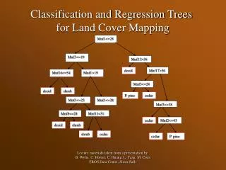
1. Classification and Regression Trees (CART)

2. Variety of approaches used • CART developed by Breiman Friedman Olsen and Stone: “Classification and Regression Trees” • C4.5 A Machine Learning Approach by Quinlan • Engineering approach by Sethi and Sarvarayudu

3. University of California- a study into patients after admission for a heart attack 19 variables collected during the first 24 hours for 215 patients (for those who survived the 24 hours) Question: Can the high risk (will not survive 30 days) patients be identified? Example

4. Answer Is the minimum systolic blood pressure over the !st 24 hours>91? Is age>62.5? H Is sinus tachycardia present? L H L

5. Features of CART • Binary Splits • Splits based only on one variable

6. Plan for Construction of a Tree • Selection of the Splits • Decisions when to decide that a node is a terminal node (i.e. not to split it any further) • Assigning a class to each terminal node

7. Impurity of a Node • Need a measure of impurity of a node to help decide on how to split a node, or which node to split • The measure should be at a maximum when a node is equally divided amongst all classes • The impurity should be zero if the node is all one class

8. Measures of Impurity • Misclassification Rate • Information, or Entropy • Gini Index In practice the first is not used for the following reasons: • Situations can occur where no split improves the misclassification rate • The misclassification rate can be equal when one option is clearly better for the next step

9. Problems with Misclassification Rate I Possible split Possible split Neither improves misclassification rate, but together give perfect classification!

10. Problems with Misclassification Rate II 400 of A 400 of B OR? 400 of A 400 of B 300 of A 100 of B 200 of A 400 of B 200 of A 0 of B 100 of A 300 of B

11. Misclassification rate for two classes 1/2 0.5 0 1 p1

12. Information • If a node has a proportion of pj of each of the classes then the information or entropy is: where 0log0 = 0 Note: p=(p1,p2,…. pn)

13. Gini Index • This is the most widely used measure of impurity (at least by CART) • Gini index is:

15. Tree Impurity • We define the impurity of a tree to be the sum over all terminal nodes of the impurity of a node multiplied by the proportion of cases that reach that node of the tree • Example i) Impurity of a tree with one single node, with both A and B having 400 cases, using the Gini Index: Proportions of the two cases= 0.5 Therefore Gini Index= 1-(0.5)2- (0.5)2 = 0.5

16. Tree Impurity Calculations

18. Selection of Splits • We select the split that most decreases the Gini Index. This is done over all possible places for a split and all possible variables to split. • We keep splitting until the terminal nodes have very few cases or are all pure – this is an unsatisfactory answer to when to stop growing the tree, but it was realized that the best approach is to grow a larger tree than required and then to prune it!

19. Example – The same one used for Nearest Neighbour classification

20. Possible Splits • There are two possible variables to split on and each of those can split for a range of values of c i.e.: x<c or x≥c And: y<c or y≥c

21. Etc.

23. Then use Data table to find the best value for a split.

26. The Next Step • You’d now need to develop a series of spreadsheets to work out the next best split • This is easier in R!

27. Developing Trees using R • Need to load the package “rpart” which contains the set of functions for CART • The function looks like: NNB.tree<-rpart(Type~., NNB[ , 1:2], cp = 1e-3) This takes the data in Type (which contains the classes for the data, i.e. A or B), and builds a model on all the variables indicated by “~.” . The data is in NNB[, 1,2] and cp is complexity parameter (more to come about this).

29. A More Complicated Example • This is based on my own research • Wish to tell which is best method of exponential smoothing to use based on the data automatically. • The variables used are the differences of the fits for three different methods (SES, Holt’s and Damped Holt’s Methods), and the alpha, beta and phi estimated for Damped Holt method.

30. This gives a very complicated tree!

31. Pruning the Tree I • As I said earlier it has been found that the best method of arriving at a suitable size for the tree is to grow an overly complex one then to prune it back. The pruning is based on the misclassification rate. However the error rate will always drop (or at least not increase) with every split. This does not mean however that the error rate on Test data will improve.

32. Source: CART by Breiman et al.

33. Pruning the Tree II • The solution to this problem is cross-validation. One version of the method carries out a 10 fold cross validation where the data is divided into 10 subsets of equal size (at random) and then the tree is grown leaving out one of the subsets and the performance assessed on the subset left out from growing the tree. This is done for each of the 10 sets. The average performance is then assessed.

34. Pruning the Tree III • This is all done by the command “rpart” and the results can be accessed using “printcp “ and “plotcp”. • We can then use this information to decide how complex (determined by the size of cp) the tree needs to be. The possible rules are to minimise the cross validation relative error (xerror), or to use the “1-SE rule” which uses the largest value of cp with the “xerror” within one standard deviation of the minimum. This is preferred by Breiman et al and B D Ripley who has included it as a dashed line in the “plotcp” function

35. > printcp(expsmooth.tree) Classification tree: rpart(formula = Model ~ Diff1 + Diff2 + alpha + beta + phi, data = expsmooth, cp = 0.001) Variables actually used in tree construction: [1] alpha beta Diff1 Diff2 phi Root node error: 2000/3000 = 0.66667 n= 3000 CP nsplit rel error xerror xstd 1 0.4790000 0 1.0000 1.0365 0.012655 2 0.2090000 1 0.5210 0.5245 0.013059 3 0.0080000 2 0.3120 0.3250 0.011282 4 0.0040000 4 0.2960 0.3050 0.011022 5 0.0035000 5 0.2920 0.3115 0.011109 6 0.0025000 8 0.2810 0.3120 0.011115 7 0.0022500 9 0.2785 0.3085 0.011069 8 0.0020000 13 0.2675 0.3105 0.011096 9 0.0017500 16 0.2615 0.3075 0.011056 10 0.0016667 20 0.2545 0.3105 0.011096 11 0.0012500 23 0.2495 0.3175 0.011187 12 0.0010000 25 0.2470 0.3195 0.011213

36. This relative CV error tends to be very flat which is why the “1-SE” Rule is preferred

38. This suggests that a cp of 0.003 is about right for this tree - giving the tree shown

39. Cost complexity • Whilst we did not use misclassification rate to decide on where to split the tree we do use it in the pruning. The key term is the relative error (which is normalised to one for the top of the tree). The standard approach is to choose a value of , and then to choose a tree to minimise R =R+ size where R is the number of misclassified points and the size of the tree is the number of end points. “cp” is /R(root tree).

40. Regression trees Trees can be used to model functions though each end point will result in the same predicted value, a constant for that end point. Thus regression trees are like classification trees except that the end pint will be a predicted function value rather than a predicted classification.

41. Measures used in fitting Regression Tree • Instead of using the Gini Index the impurity criterion is the sum of squares, so splits which cause the biggest reduction in the sum of squares will be selected. • In pruning the tree the measure used is the mean square error on the predictions made by the tree.

42. Regression Example • In an effort to understand how computer performance is related to a number of variables which describe the features of a PC the following data was collected: the size of the cache, the cycle time of the computer, the memory size and the number of channels (both the last two were not measured but minimum and maximum values obtained).

43. This gave the following tree:

44. We can see that we need a cp value of about 0.008 - to give a tree with 11 leaves or terminal nodes

45. This enables us to see that, at the top end, it is the size of the cache and the amount of memory that determine performance

46. Advantages of CART • Can cope with any data structure or type • Classification has a simple form • Uses conditional information effectively • Invariant under transformations of the variables • Is robust with respect to outliers • Gives an estimate of the misclassification rate

47. Disadvantages of CART • CART does not use combinations of variables • Tree can be deceptive – if variable not included it could be as it was “masked” by another • Tree structures may be unstable – a change in the sample may give different trees • Tree is optimal at each split – it may not be globally optimal.

48. Exercises • Implement Gini Index on a spreadsheet • Have a go at the lecture examples using R and the script available on the web • Try classifying the Iris data using CART.