Download
1 / 31
450 likes | 1.27k Views
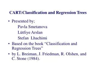
CART:Classification and Regression Trees. Presented by; Pavla Smetanova Lütfiye Arslan Stefan Lhachimi Based on the book “Classification and Regression Trees” by L. Breiman, J. Friedman, R. Olshen, and C. Stone (1984). Outline. 1- INTRODUCTION What is CART ? An example

E N D
CART:Classification and Regression Trees • Presented by; Pavla Smetanova Lütfiye Arslan Stefan Lhachimi • Based on the book “Classification and Regression Trees” • by L. Breiman, J. Friedman, R. Olshen, and C. Stone (1984).
Outline 1- INTRODUCTION • What is CART? • An example • Terminology • Strengths 2- METHOD:3 steps in CART: • Tree building • Pruning • The final tree
What is CART? • A non-parametric technique,using the methodology of tree building. • Classifies objects or predicts outcomes by selecting from a large number of variables the most important ones in determining the outcome variable. • CART analysis is a form of binary recursive partitioning.
An example from Clinical research • Development of a reliable clinical decision rule to classify new patients into categories • 19 measurements(age, blood pressure, etc.)are taken from each heart-attack patients during the first 24 hours of their admittance to San Diego Hospital. • The goal: identify high-risk patients
Classification of Patients as High or No risk groups Is the minimum systolic blod pressure over the initial 24 hour> 91? yes no Is age>62.5? yes no Is sinus tachycardia present? yesno G F G F
Terminology • The classification problem: A systematic way of predicting the class of an object based on measurements. • C={1,...,J}: classes • x: measurement vector • d(x): a classifying function assigning every x to one of the classes 1,...,J.
Terminology • s: split • learning sample (L): measurement data on N cases observed in the past together with their actual classification. • R*(d): true misclassification rate R*(d)=P(d(x)=Y), Y C
Strengths • No distributional assumptions are required. • No assumption of homogeneity. • The explanatory variables can be a mixture of categorical, interval and continuous. • Especially good for high-dimensional and large data sets. Produce useful results by using a few important variables.
Strengths • Sophisticated methods for dealing with missing variables. • Unaffected by outliers, collinearities, heteroscedascity. • Not difficult to interpret. • An important weakness: Not based on a probabilistic model, no confidence interval.
Dealing with Missing values • CART does not drop cases with missing measurement values. • Surrogate Splits: Define a measurement of similarity between any two splits s, s´ of t. • If best split of t is s on varible xm, find s´ on other variables that is most similar to s. Call it best surrogateof s. Find 2nd best, so on... • If a case has xm missing, refer to surrogates.
3 Steps in CART • Tree building • Pruning • Optimal tree selection If the dependent variable is categorical then a classification tree and if it is continuous regression trees are used. • Remark: Until the Regression part, we talk just about classification trees.
Example Tree 1 = root node = terminal node = non-terminal
Tree Building Process • What is a tree? The collection of repeated splits of subsets of X into two descendant subsets. • A finite non-empty set T and two functions left(.) and right(.) from t to T which satisfy; • For each t T, either left(t)=right(t)=0,or left(t)>t and right(t)>t • For each t T, other than the smallest integer in T, there is exactly one s T s.t. either t=left(s) or t=right(s).
Terminology of tree • root of T: the minimum element of a tree • s: parentof T, if t=left(s) or t=right(s), t: child • T*: set of terminal nodes: left(t)=right(t)=0. • T-T*: non-terminal nodes • A node s is ancestor of t if s=parent(t) or s=parent(parent(t)) or...
A node tis descendant of s, if s is an ancestor of t. • A branch of Tt of T with root node t T consists of the node t and all descendants of t in T. • The main problem of tree building: how to use the data L to determine the splits, the terminal nodes and assignment of terminals to classes.
Steps of tree building • Start with splitting a variable at all of its split points. Sample splits into two binary nodes at each split point. • Select the best split in the variable in terms of the reduction in impurity (heterogeneity) • Repeat steps 1,2 for all variables at the root node.
Rank all of the best splits and select the variable that achieves the highest purity at root. • Assign classes to the nodes according to a rule that minimizes misclassification costs. • Repeat 1-5 for each non-terminal node • Grow a very large tree Tmax until all terminal nodes are either small or pure or contain identical measurement vectors. • Prune and choose final tree using the cross validation.
1-2 Construction of the classifier • Goal: find a split, s , that divides L intoso pure as possible subsets. • Goodness of split criteria is the decrease in impurity: i(s,t)=i(t)-pLi(tL)- pRi(tR). where i(t):node impurity, pL,pR;proportion of the cases that has been split to the left or right.
To extract the best split, choose the s* which fulfills; i(s*,t)=maxs i(s,t) • Repeat the same till a node t is reached(optimization at each step) such that no significant decrease in purity is possible, declare it then as terminal node.
5-Estimating accuracy • Concept of R*(d): Construct d usingL. Draw another sample from the same population as L. Observe the correct classification, find the predicted classification using d(x). • The proportion misclassified by d is the value of R*(d).
3 internal estimates of R*(d) • The resubstitution estimate(least accurate) R(d)=1/N nI(d(xn)jn). • Test-sample estimate: (for large sample sizes) Rts(d)=1/N2(xn,jn)I(d(xn) jn). • Cross-validation(preferred for smaller samples) Rts(d(v))=1/Nv(xn,jn)I(d(v)(xn) jn). RCV(d)=1/VvRts(d(v)).
7-Before Pruning • Instead of finding appropriate stopping rules, grow a Tmaxand prune it to the root. Then use R*(T) to select the optimal tree among pruned subtrees. • Before pruning, for growing a sufficiently large initial tree Tmax specifies Nmin and split until each terminal node either is pure or N(t)Nmin. • Generally Nmin has been set at 5, occasionally at 1.
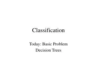
Tree T-T2 Tree T Branch T2 Definition : Pruning a branch Tt from a tree T consists of deleting all descendants of t except its root node. T- Tt is the pruned tree.
Minimal Cost-Complexity Pruning • For any subtree T Tmax, complexity |T| :the number of terminal nodes in T. • Let 0, be a real number called the complexity parameter, a measure of how much additional accuracy a split must add to the entire tree to warrant the additional complexity. • The cost-complexity measure R(T) is a linear combination of the cost of the tree and its complexity. R (T)=R(T)+ |T| .
For each value of α, find the subtree T() which minimizes R (T),i.e., R (T())=minT R (T). • For =0, we have the Tmax. As increases the tree become smaller, reducing down to the root at the extreme. • Result is a finite sequence of subtrees T1, T2, T3 ,... Tk with progressively fewer terminal nodes.
Optimal Tree Selection • Task: find the correct complexity parameter so that the information in L is fit, but not overfit. • This requires normally an independent set of data. If not available, use CROSS-Validationto pick out that subtree with the lowest estimated misclassification rate.
Cross-Validation • L randomly divided into V subsets, L1,..., LV. • For every v=1,...,V; apply the procedure using L- LV as a learning sample and let d(v)(x) be the resulting classifier. A test sample estimate for R*(d(v)) is; Rts(d(v))=1/Nv(xn,jn)I(d(v)(xn) jn). where Nvis the number of cases in LV.
Regression trees • The basic idea same with classification. The regression estimator in the first step; • The regression estimator in the second step;
Split R into R1 and R2 such that sum of squared residuals of the estimator is minimized; which is the counterpart of true misclassification rate in classification trees.
Comments • Mostly used in clinical research, air pollution, criminal justice, molecular structures,... • More accurate on nonlinear problems compared to linear regression. • look at the data from different viewpoints.