Download
1 / 58
690 likes | 1.35k Views
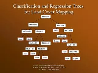
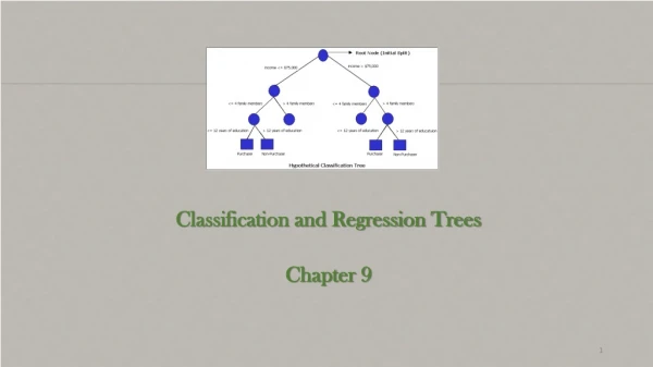
Classification and regression trees. Pierre Geurts Stochastic methods (Prof. L.Wehenkel) University of Liège. Outline. Supervised learning Decision tree representation Decision tree learning Extensions Regression trees By-products. Database.

E N D
Classification and regression trees Pierre Geurts Stochastic methods (Prof. L.Wehenkel) University of Liège
Outline • Supervised learning • Decision tree representation • Decision tree learning • Extensions • Regression trees • By-products
Database • A collection of objects (rows) described by attributes (columns)
Supervised learning inputs output • Goal: from the database, find a function f of the inputs that approximate at best the output • Discrete output classification problem • Continuous output regression problem Automatic learning Ŷ = f(A1,A2,…,An) model Database=learning sample
Examples of application (1) • Predict whether a bank client will be a good debtor or not • Image classification: • Handwritten characters recognition: • Face recognition 3 5
Examples of application (2) • Classification of cancer types from gene expression profiles (Golub et al (1999))
1 A2 A model(h H) obtained by automatic learning 0 0 1 A1 Learning algorithm • It receives a learning sample and returns a function h • A learning algorithm is defined by: • A hypothesis space H (=a family of candidate models) • A quality measure for a model • An optimisation strategy
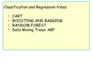
Decision (classification) trees • A learning algorithm that can handle: • Classification problems (binary or multi-valued) • Attributes may be discrete (binary or multi-valued) or continuous. • Classification trees were invented twice: • By statisticians: CART (Breiman et al.) • By the AI community: ID3, C4.5 (Quinlan et al.)
Hypothesis space • A decision tree is a tree where: • Each interior node tests an attribute • Each branch corresponds to an attribute value • Each leaf node is labelled with a class A1 a13 a11 a12 A3 A2 c1 a32 a31 a21 a22 c1 c2 c2 c1
Outlook Rain Sunny Overcast Wind Humidity yes Weak Strong High Normal yes no yes no A decision tree for playtennis
Outlook Rain Sunny Overcast Wind Humidity yes Weak Strong High Normal yes no yes no Tree learning • Tree learning=choose the tree structure and determine the predictions at leaf nodes • Predictions: to minimize the misclassification error, associate the majority class among the learning sample cases reaching this node 25 yes, 40 no 15 yes, 10 no 14 yes, 2 no
How to generate trees ? (1) • What properties do we want the decision tree to have ? • It should be consistent with the learning sample (for the moment) • Trivial algorithm: construct a decision tree that has one path to a leaf for each example • Problem: it does not capture useful information from the database
How to generate trees ? (2) • What properties do we want the decision tree to have ? • It should be at the same time as simple as possible • Trivial algorithm: generate all trees and pick the simplest one that is consistent with the learning sample. • Problem: intractable, there are too many trees
Top-down induction of DTs (1) • Choose « best » attribute • Split the learning sample • Proceed recursively until each object is correctly classified Outlook Rain Sunny Overcast
Top-down induction of DTs (2) Procedure learn_dt(learning sample, LS) • If all objects from LS have the same class • Create a leaf with that class • Else • Find the « best » splitting attribute A • Create a test node for this attribute • For each value a of A • BuildLSa= {oLS | A(o) is a} • Use Learn_dt(LSa) to grow a subtree from LSa.
Properties of TDIDT • Hill-climbing algorithm in the space of possible decision trees. • It adds a sub-tree to the current tree and continues its search • It does not backtrack • Sub-optimal but very fast • Highly dependent upon the criterion for selecting attributes to test
Which attribute is best ? • We want a small tree • We should maximize the class separation at each step, i.e. make successors as pure as possible • it will favour short paths in the trees A1=? [29+,35-] A2=? [29+,35-] T F T F [21+,5-] [8+,30-] [18+,33-] [11+,2-]
Impurity • Let LS be a sample of objects, pj the proportions of objects of class j(j=1,…,J) in LS, • Define an impurity measure I(LS) that satisfies: • I(LS) is minimum only when pi=1 and pj=0 for ji (all objects are of the same class) • I(LS) is maximum only when pj =1/J (there is exactly the same number of objects of all classes) • I(LS) is symmetric with respect to p1,…,pJ
| LS | å = - a I ( LS , A ) I ( LS ) I ( LS ) D a | LS | a Reduction of impurity • The “best” split is the split that maximizes the expected reduction of impurity whereLSa is the subset of objects from LS such that A=a. • I is called a score measure or a splitting criterion • There are many other ways to define a splitting criterion that do not rely on an impurity measure
Example of impurity measure (1) • Shannon’s entropy: • H(LS)=-åj pj log pj • If two classes, p1=1-p2 • Entropy measures impurity, uncertainty, surprise… • The reduction of entropy is called the information gain
Example of impurity measure (2) • Which attribute is best ? A1=? [29+,35-] A2=? [29+,35-] I=0.99 I=0.99 T F T F [21+,5-] [8+,30-] [18+,33-] [11+,2-] I=0.71 I=0.75 I=0.94 I=0.62 • I(LS,A1) = 0.99 - (26/64) 0.71 – (38/64) 0.75 = 0.25 • I(LS,A2) = 0.99 - (51/64) 0.94 – (13/64) 0.62 = 0.12
Other impurity measures • Gini index: • I(LS)=åjpj (1-pj) • Misclassification error rate: • I(LS)=1-maxj pj • two-class case:
Playtennis problem Outlook Rain • Which attribute should be tested here ? • I(LS,Temp.) = 0.970 - (3/5) 0.918 - (1/5) 0.0 - (1/5) 0.0=0.419 • I(LS,Hum.) = 0.970 - (3/5) 0.0 - (2/5) 0.0 = 0.970 • I(LS,Wind) = 0.970 - (2/5) 1.0 - (3/5) 0.918 = 0.019 • the best attribute is Humidity Sunny Overcast
Overfitting (1) • Our trees are perfectly consistent with the learning sample • But, often, we would like them to be good at predicting classes of unseen data from the same distribution (generalization). • A tree T overfits the learning sample iff T’ such that: • ErrorLS(T) < ErrorLS(T’) • Errorunseen(T) > Errorunseen(T’)
Overfitting (2) Error • In practice, Errorunseen(T) is estimated from a separate test sample Overfitting Underfitting Errorunseen ErrorLS Complexity
Temperature Outlook Rain Sunny Mild Cool,Hot Overcast Wind Humidity no yes yes Weak Strong High Normal yes no yes yes no Add a test here Reasons for overfitting (1) • Data is noisy or attributes don’t completely predict the outcome
area with probably wrong predictions Reasons for overfitting (2) • Data is incomplete (not all cases covered) • We do not have enough data in some part of the learning sample to make a good decision - + + + - + - + - + - + - - + - - - - - - - - - - - -
How can we avoid overfitting ? • Pre-pruning: stop growing the tree earlier, before it reaches the point where it perfectly classifies the learning sample • Post-pruning: allow the tree to overfit and then post-prune the tree • Ensemble methods (this afternoon)
Pre-pruning • Stop splitting a node if • The number of objects is too small • The impurity is low enough • The best test is not statistically significant (according to some statistical test) • Problem: • the optimum value of the parameter (n, Ith , significance level) is problem dependent. • We may miss the optimum
Post-pruning (1) • Split the learning sample LS into two sets: • a growing sample GS to build the tree • A validation sample VS to evaluate its generalization error • Build a complete tree from GS • Compute a sequence of trees {T1,T2,…} where • T1 is the complete tree • Ti is obtained by removing some test nodes from Ti-1 • Select the tree Ti* from the sequence that minimizes the error on VS
Overfitting Underfitting Tree puning Error on VS Error on GS Tree growing Optimal tree Post-pruning (2) Error Complexity
Post-pruning (3) • How to build the sequence of trees ? • Reduced error pruning: • At each step, remove the node that most decreases the error on VS • Cost-complexity pruning: • Define a cost-complexity criterion: • ErrorGS(T)+a.Complexity(T) • Build the sequence of trees that minimize this criterion for increasing a
Outlook Rain Sunny Overcast no yes yes Outlook Rain Sunny Overcast Wind Humidity yes Weak Strong High Normal Outlook Rain no yes no Temp. Sunny Overcast Cool,Hot Mild Wind Humidity yes no yes yes Weak Strong High Normal yes no yes no Outlook Rain Sunny Overcast Wind no yes Weak Strong yes no Post-pruning (4) T1 T3 ErrorGS=13%, ErrorVS=15% ErrorGS=0%, ErrorVS=10% T4 T2 ErrorGS=27%, ErrorVS=25% T5 ErrorGS=6%, ErrorVS=8% ErrorGS=33%, ErrorVS=35%
Post-pruning (5) • Problem: require to dedicate one part of the learning sample as a validation set may be a problem in the case of a small database • Solution: N-fold cross-validation • Split the training set into N parts (often 10) • Generate N trees, each leaving one part among N • Make a prediction for each learning object with the (only) tree built without this case. • Estimate the error of this prediction • May be combined with pruning
How to use decision trees ? • Large datasets (ideal case): • Split the dataset into three parts: GS, VS, TS • Grow a tree from GS • Post-prune it from VS • Test it on TS • Small datasets (often) • Grow a tree from the whole database • Pre-prune with default parameters (risky), post-prune it by 10-fold cross-validation (costly) • Estimate its accuracy by 10-fold cross-validation
Outline • Supervised learning • Tree representation • Tree learning • Extensions • Continuous attributes • Attributes with many values • Missing values • Regression trees • By-products
Temperature 65.4 >65.4 no yes Continuous attributes (1) • Example: temperature as a number instead of a discrete value • Two solutions: • Pre-discretize: Cold if Temperature<70, Mild between 70 and 75, Hot if Temperature>75 • Discretize during tree growing: • How to find the cut-point ?
Temp. Play 64 Yes Temp.< 68.5 I=0.000 Temp.< 80.5 I=0.000 Temp.< 69.5 I=0.015 Temp.< 70.5 I=0.045 Temp.< 73.5 I=0.001 Temp.< 71.5 I=0.001 Temp.< 64.5 I=0.048 Temp.< 82 I=0.010 Temp.< 84 I=0.113 Temp.< 66.5 I=0.010 Temp.< 77.5 I=0.025 65 No 68 Yes 69 Yes 70 Yes 71 No Sort 72 No 72 Yes 75 Yes 75 Yes 80 No 81 Yes 83 Yes 85 No Continuous attributes (2)
A2<0.33 ? yes no good A1<0.91 ? A2<0.91 ? A1<0.23 ? 1 good bad A2<0.75 ? A2<0.49 ? A2 good bad bad A2<0.65 ? 0 0 1 A1 bad good Continuous attribute (3)
Attributes with many values (1) Letter • Problem: • Not good splits: they fragment the data too quickly, leaving insufficient data at the next level • The reduction of impurity of such test is often high (example: split on the object id). • Two solutions: • Change the splitting criterion to penalize attributes with many values • Consider only binary splits (preferable) a y z c b …
Attributes with many values (2) • Modified splitting criterion: • Gainratio(LS,A)= H(LS,A)/Splitinformation(LS,A) • Splitinformation(LS,A)=-åa |LSa|/|LS| log(|LSa|/|LS|) • The split information is high when there are many values • Example: outlook in the playtennis • H(LS,outlook) = 0.246 • Splitinformation(LS,outlook) = 1.577 • Gainratio(LS,outlook) = 0.246/1.577=0.156 < 0.246 • Problem: the gain ratio favours unbalanced tests
Attributes with many values (3) • Allow binary tests only: • There are 2N-1 possible subsets for N values • If N is small, determination of the best subsets by enumeration • If N is large, heuristics exist (e.g. greedy approach) Letter {a,d,o,m,t} All other letters
Missing attribute values • Not all attribute values known for every objects when learning or when testing • Three strategies: • Assign most common value in the learning sample • Assign most common value in tree • Assign probability to each possible value
Regression trees (1) • Tree for regression: exactly the same model but with a number in each leaf instead of a class Outlook Rain Sunny Overcast Wind Humidity 45.6 Weak Strong High Normal Temperature 7.4 64.4 22.3 <71 >71 1.2 3.4
r5 r4 r3 r2 r1 Regression trees (2) • A regression tree is a piecewise constant function of the input attributes X2 X1 t1 r5 r2 X1 t3 X2 t2 r3 t2 r4 r1 X2 t4 t3 t1 X1
| LS | å D = - a I ( LS , A ) var { y } var { y } | | y LS y LS | LS | a a Regression tree growing • To minimize the square error on the learning sample, the prediction at a leaf is the average output of the learning cases reaching that leaf • Impurity of a sample is defined by the variance of the output in that sample: I(LS)=vary|LS{y}=Ey|LS{(y-Ey|LS{y})2} • The best split is the one that reduces the most variance:
Regression tree pruning • Exactly the same algorithms apply: pre-pruning and post-pruning. • In post-pruning, the tree that minimizes the squared error on VSis selected. • In practice, pruning is more important in regression because full trees are much more complex (often all objects have a different output values and hence the full tree has as many leaves as there are objects in the learning sample)
Outline • Supervised learning • Tree representation • Tree learning • Extensions • Regression trees • By-products • Interpretability • Variable selection • Variable importance
Outlook Rain Sunny Overcast Wind Humidity yes Weak Strong High Normal yes no yes no Interpretability (1) • Obvious • Compare with a neural networks: Outlook Play Humidity Wind Don’t play Temperature