Download
1 / 58
640 likes | 765 Views
Chapter 10 Correlation and Regression. 10-2 Correlation (Part 1 Only) 10-3 Regression (Part 1 Only). Preview.

E N D
Chapter 10Correlation and Regression 10-2 Correlation (Part 1 Only) 10-3 Regression (Part 1 Only)
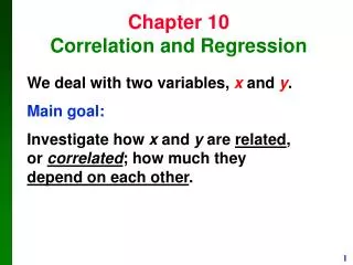
Preview In this chapter we introduce methods for determining whether a correlation, or association, between two variables exists and whether the correlation is linear. For linear correlations, we can identify an equation that best fits the data and we can use that equation to predict the value of one variable given the value of the other variable.
Section 10-2 Correlation
Key Concept Part 1 of this section introduces the linear correlation coefficient r, which is a numerical measure of the strength of the relationship between two variables representing quantitative data. Using paired sample data (sometimes called bivariate data), we find the value of r (usually using technology), then we use that value to conclude that there is (or is not) a linear correlation between the two variables.
Key Concept In this section we consider only linear relationships, which means that when graphed, the points approximate a straight-line pattern.
Definition A correlation exists between two variables when the values of one are somehow associated with the values of the other in some way.
Definition The linear correlation coefficientr measures the strength of the linear relationship between the paired quantitative x- and y-values in a sample.
Exploring the Data We can often see a relationship between two variables by constructing a scatterplot. Figure 10-2 following shows scatterplots with different correlation coefficients.
Scatterplots of Paired Data Figure 10-2
Scatterplots of Paired Data Figure 10-2
Scatterplots of Paired Data Figure 10-2
Example: problem 10 on page 509 • Construct a scatterplot
Scatterplot with Graphing Calculator • Enter the X data values in two lists. • Press 2nd STATPLOT and choose #1 PLOT 1. Be sure the plot is ON, the scatter plot icon is highlighted (top row, first icon) • Enter the list of the X data values next to Xlist, and the list of the Y data values next to Ylist. • Choose any of the three marks. Press ZOOM and #9 ZoomStat.
Example: problem 10 on page 509 • Scatterplot • Note the outlier at x=13
Properties of the Linear Correlation Coefficient r 1. –1 r 1 2. if all values of either variable are converted to a different scale, the value of r does not change. 3. the value of r is not affected by the choice of x and y. Interchange all x- and y-valuesand the value of r will not change. 4. r measures strength of a linear relationship (the closer r is to positive or negative 1, the “more linear” the relationship)
nxy–(x)(y) r= n(x2)– (x)2n(y2)– (y)2 Formula For r The linear correlation coefficientr measures the strength of a linear relationship between the paired values in a sample. Formula 10-1 Computer software or calculators can compute r
Notation for the Linear Correlation Coefficient n = number of pairs of sample data denotes the addition of the items indicated. x denotes the sum of all x-values. x2 indicates that each x-value should be squared and then those squares added. (x)2 indicates that the x-values should be added and then the total squared.
Notation for the Linear Correlation Coefficient xy indicates that each x-value should be first multiplied by its corresponding y-value. After obtaining all such products, find their sum. r = linear correlation coefficient for sample data. = linear correlation coefficient for population data.
Example: problem 10 on page 509 • Find the linear correlation coefficient r and determine if there is sufficient evidence to support the claim of a linear correlation between x and y.
Calculate r Using Calculator • (see page 508 of your book) • Enter the data in two lists. • Press STAT and select TESTS • LinRegTTest is option F (scroll arrow up 3 places) • Enter the names of the lists from step 1. • Arrow down to Calculate and then press Enter • The r value is the last value displayed; round this value to three decimal places
Calculate r Using Calculator • Example: problem 10 on page 509 • Using calculator we find that r = 0.816
Interpreting r • Using Table A-5: • Find the row with same value of n as the data set • If the absolute value of the computed value of r, denoted |r|, is greater than the number in the first column in Table A-5, conclude that there is a linear correlation. Otherwise, there is not sufficient evidence to support the conclusion of a linear correlation.
Table A-5 • For n=11 critical value of r is 0.602
Interpret r • Example: problem 10 on page 509 (b) Comparing 0.602 with r = 0.816, there is a (positive) linear correlation since r is greater than 0.602
Interpret r • Example: problem 10 on page 509 (c) Identify the feature of the data that would be missed if part (b) was completed without the use of a scatterplot ANSWER: scatterplot shows the relationship is linear except for one point (an error or an outlier at x=13)
Properties of the Linear Correlation Coefficient r r is very sensitive to outliers, they can dramatically affect its value. If (13,12.74) is removed from the list in the previous example, the calculator gives r = 0.999996554
Interpret r • NOTE: if r is negative, take its absolute value before comparing with value in Table A-5 • Example: r = -0.375 and n=17 From Table A-5, for n=17 we get a value of 0.482 Comparing |r|=0.375 there is not evidence for a linear correlation since |r| is less than 0.482
Caution Know that the methods of this section apply to a linear correlation. If you conclude that there does not appear to be linear correlation, know that it is possible that there might be some other association that is not linear.
Interpreting r:Explained Variation The value of r2 is the proportion of the variation in y that is explained by the linear relationship between x and y.
Example: Using example problem 10 on page 509, the linear correlation coefficient was r = 0.816. The proportion of y can be explained by the variation in x: r2 =(0.816)(0.816)=0.666 We conclude that 0.666 (or about 67%) of the variation in y can be explained by the variation in x. This implies that about 33% of the variation in y cannot be explained by the variation in x.
Common Errors Involving Correlation 1. Causation: It is wrong to conclude that correlation implies causality. 2. Averages: Averages suppress individual variation and may inflate the correlation coefficient. 3. Linearity: There may be some relationship between x and y even when there is no linear correlation.
Recap • In this section, we have discussed: • Correlation. • The linear correlation coefficient r. • Requirements, notation and formula for r. • Interpreting r.
Section 10-3 Regression
Key Concept In part 1 of this section we find the equation of the straight line that best fits the paired sample data. That equation algebraically describes the relationship between two variables. The best-fitting straight line is called a regression line and its equation is called the regression equation.
Regression The regression equation expresses a relationship between x (called the explanatory variable, predictor variable or independent variable), and y (called the response variable or dependent variable). ^
Definitions Regression Equation ^ y= b0 + b1x Given a collection of paired data, the regression equation algebraically describes the relationship between the two variables. • Regression Line • The graph of the regression equation is called the regression line (or line of best fit, or leastsquares line).
The regression line is the best linear fit of the sample points. Special Property
Regression The typical equation of a straight line: m = slope of the line (coefficient of x) b = y-intercept of the line (constant) y = m x + b
Notation for Regression Equation (Sample) y-intercept of regression equation Slope of regression equation Equation of the regression line b0 b1 y = b0 + b1x ^ Sample Statistic
Notation for Regression Equation (Population) y-intercept of regression equation Slope of regression equation Equation of the regression line Population Parameter 0 1 y = 0 + 1x
Requirements 1. The sample of paired (x, y) data is a random sample of quantitative data. 2. Visual examination of the scatterplot shows that the points approximate a straight-line pattern. 3. Any outliers must be removed if they are known to be errors. Consider the effects of any outliers that are not known errors.
Formulas for b0 and b1 calculators or computers can compute these values (round to three significant digits) (slope) Formula 10-3 (y-intercept) Formula 10-4
Calculator Enter the data in two lists. Make a scatter plot of the data (use 2nd Y= to get STAT PLOT, choose Plot1 On, first scatterplot icon, then zoom 9) (your plot will look different)
Calculator 3. Plot the regression line. Choose: 4. STAT → CALC #4 LinReg(ax+b) Include the parameters L1, L2, Y1. NOTE: Y1 comes from VARS → YVARS, #Function, Y1
Calculator Choose Y= and the equation for the regression line will be stored in Y1Then choose GRAPH and the regression line will be plotted.
Calculator 6. Choose TRACE and you can see X and Y values on scatterplot or regression line
Calculate Regression Line • Example: problem 10 on page 526
Calculate Regression Line • Example: problem 10 on page 526 • Scatterplot