Download
1 / 20
210 likes | 305 Views
Chapter 4 – Correlation and Regression. before: examined relationship among 1 variable (test grades, metabolism, trip time to work, etc.). now: will examine relationship between 2 variables (study time and test grades, age and metabolism, trip time to work and distance to work, etc.).

E N D
Chapter 4 – Correlation and Regression before: examined relationship among 1 variable (test grades, metabolism, trip time to work, etc.) now: will examine relationship between 2 variables (study time and test grades, age and metabolism, trip time to work and distance to work, etc.)
The 2 Variables • Response variable – measures an outcome of a study • Explanatory variable – explains or influences changes in a response variable • Ex. y=2x+4 • explanatory: x response: y Ex. The number of hours you study and the grade you earn explanatory: hours studied response: grade Ex. Safety training hours at an industrial plant and the number of work hours lost due to accidents. explanatory: traininghours response: work hours
Ways to examine 2 variables • Form – shape (linear, exponential, parabola, none) • Direction – positive or negative slope • Strength – how tight do the points fit the line of best fit Terminology: graph “y against x” means:
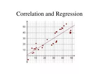
Scatter plot • Shows relationship between two quantitative variables • Each dot represents an individual data point (x,y) Positive Negative None
Strength & Direction of Linear Relationship • Measured by the correlation coefficient; r • Expanding this formula for 3 data points yields:
Facts about r • Value is always between: -1 and 1 • If r is negative, then there is a negative relationship • If r is positive, then there is a positive relationship • If r = -1 or r = 1, then all points lie on a straight line
Facts about r • Strength of correlation: • Values close to -1 or 1 signify a strong linear rel. • If r = -1 or r = 1, then all points lie on a straight line • Values close to 0 signify a weak linear rel. For the sake of this class -1 -0.9 -0.7 0 0.7 0.9 1 Moderate Strong Moderate Strong Weak
Lurking Variables • Def: neither explanatory or response, but may be responsible for changes in these variables. • Ex. In the past few years, the population of Lynchburg has increased. It was observed that during this time there was a correlation between the number of people attending church and the number of people in jail. • Hopefully church attendance doesn’t cause people to go to jail. • Lurking Variable – population growth
Facts continued • No distinction between explanatory and response variable (you will get the same r value if you swap the two variables) • r has no unit • Not resistant to outliers • Is not a complete description of two-variables
Least squares regression line(LSRL) • Makes the sum of the square distances of the vertical lines the smallest • Used to predict the value of y.
How to find this line • Recall: any line • Regression line: **** USE CAUTION WITH THE “b” ****
Example • Make a scatter plot on your calculator. • Find the equation for the regression line and then graph it on your scatter plot. • What may be a good list price for a 1,700 sq ft home? 2,500 sq ft home?
Facts about LSRL • Distinction between explanatory and response different than • Even though graphs will change the value for the regression r, will not. • Close connection between slope and correlation
LSRL Facts continued • LSRL always passes through point: • r2 is a measure of the proportion of variation that is explained by the regression line. • “how much of r is explained by the points” • if r = -0.74 then r2 = 0.56 which means that 56% of the variations are accounted for by the LSRL.
Residuals • Residual = observed value – predicted value • If residual is a positive (+) number, point is above line • If residual is a negative (-) number, point is below line • The mean of residuals is always zero
Extrapolation • Def: Use of LSRL to predict results outside the range of values used to calculate the LSRL • Such predictions are not accurate • Ex. • Predict the value of y when x=10 • Since you used x-values of 1-4 to find the LSRL, it is not accurate to predict what y will be at an x-value of 10.
Association does not imply causation • No cause and effect. Changes in explanatory variable (x) will not always cause changes in response variable (y) • Ex. The more TV’s a country has, the longer people live. So to improve the life expectancy in other countries ship more TV’s to them.
HW • Pg 144 #’s: 1,2,5,6,13b,14b,16b,17b,20c • Pg 160 #’s: 3,9-12 parts ce, 18cf • Excel: create a scatter plot with trend line and r2 of data in guided exercise 4 on page 157. Directions are on page 159.