Download
1 / 94
940 likes | 1.03k Views
Explore the correlation between variables, calculate the linear correlation coefficient, and interpret relationships in a statistical context. Learn the properties and use of the correlation coefficient in data analysis.

E N D
9-1 Overview 9-2 Correlation 9-3 Regression 9-4 Variation and Prediction Intervals 9-5 Multiple Regression 9-6 Modeling Chapter 9Correlation and Regression Chapter 9, Triola, Elementary Statistics, MATH 1342
Section 9-1 & 9-2 Overview and Correlation and Regression Created by Erin Hodgess, Houston, Texas Chapter 9, Triola, Elementary Statistics, MATH 1342
Paired Data (p.506) Is there a relationship? If so, what is the equation? Use that equation for prediction. Overview Chapter 9, Triola, Elementary Statistics, MATH 1342
A correlation exists between two variables when one of them is related to the other in some way. Definition Chapter 9, Triola, Elementary Statistics, MATH 1342
A Scatterplot (or scatter diagram) is a graph in which the paired (x, y) sample data are plotted with a horizontal x-axis and a vertical y-axis. Each individual (x, y) pair is plotted as a single point. Definition Chapter 9, Triola, Elementary Statistics, MATH 1342
Scatter Diagram of Paired Data (p.507) Chapter 9, Triola, Elementary Statistics, MATH 1342
Positive Linear Correlation (p.498) Figure 9-2 Scatter Plots Chapter 9, Triola, Elementary Statistics, MATH 1342
Negative Linear Correlation Figure 9-2 Scatter Plots Chapter 9, Triola, Elementary Statistics, MATH 1342
No Linear Correlation Figure 9-2 Scatter Plots Chapter 9, Triola, Elementary Statistics, MATH 1342
Definition (p.509) The linear correlation coefficient r measures strength of the linear relationship between paired x and y values in a sample. Chapter 9, Triola, Elementary Statistics, MATH 1342
1. The sample of paired data (x, y) is a random sample. 2. The pairs of (x, y) data have a bivariate normal distribution. Assumptions (p.507) Chapter 9, Triola, Elementary Statistics, MATH 1342
n = number of pairs of data presented denotes the addition of the items indicated. x denotes the sum of all x-values. x2 indicates that each x-value should be squared and then those squares added. (x)2 indicates that the x-values should be added and the total then squared. xy indicates that each x-value should be first multiplied by its corresponding y-value. After obtaining all such products, find their sum. r represents linear correlation coefficient for a sample represents linear correlation coefficient for a population Notation for the Linear Correlation Coefficient Chapter 9, Triola, Elementary Statistics, MATH 1342
Definition The linear correlation coefficientr measures the strength of a linear relationship between the paired values in a sample. nxy–(x)(y) r= n(x2)– (x)2n(y2)– (y)2 Formula 9-1 Calculators can compute r (rho) is the linear correlation coefficient for all paired data in the population. Chapter 9, Triola, Elementary Statistics, MATH 1342
Round to three decimal places so that it can be compared to critical values in Table A-6. (see p.510) Use calculator or computer if possible. Rounding the Linear Correlation Coefficient r Chapter 9, Triola, Elementary Statistics, MATH 1342
Data x 1 2 1 8 3 6 5 4 y Calculating r This data is from exercise #7 on p.521. Chapter 9, Triola, Elementary Statistics, MATH 1342
Calculating r Chapter 9, Triola, Elementary Statistics, MATH 1342
Data x 1 2 1 8 3 6 5 4 y Calculating r nxy–(x)(y) r= n(x2)– (x)2n(y2)– (y)2 4(48)–(10)(20) r= 4(36)– (10)24(120)– (20)2 –8 r= = –0.135 59.329 Chapter 9, Triola, Elementary Statistics, MATH 1342
If the absolute value of r exceeds the value in Table A - 6, conclude that there is a significant linear correlation. Otherwise, there is not sufficient evidence to support the conclusion of significant linear correlation. Interpreting the Linear Correlation Coefficient (p.511) Chapter 9, Triola, Elementary Statistics, MATH 1342
Example: Boats and Manatees Given the sample data in Table 9-1, find the value of the linear correlation coefficient r, then refer to Table A-6 to determine whether there is a significant linear correlation between the number of registered boats and the number of manatees killed by boats. Using the same procedure previously illustrated, we find that r = 0.922. Referring to Table A-6, we locate the row for which n=10. Using the critical value for =5, we have 0.632. Because r = 0.922, its absolute value exceeds 0.632, so we conclude that there is a significant linear correlation between number of registered boats and number of manatee deaths from boats. Chapter 9, Triola, Elementary Statistics, MATH 1342
1. –1 r 1 (see also p.512) 2. Value of r does not change if all values of either variable are converted to a different scale. 3. The r is not affected by the choice of x and y. interchange x and y and the value of r will not change. 4. r measures strength of a linear relationship. Properties of the Linear Correlation Coefficient r Chapter 9, Triola, Elementary Statistics, MATH 1342
Interpreting r: Explained Variation The value of r2 is the proportion of the variation in y that is explained by the linear relationship between x and y. (p.503 and p.533) Chapter 9, Triola, Elementary Statistics, MATH 1342
Example: Boats and Manatees Using the boat/manatee data in Table 9-1, we have found that the value of the linear correlation coefficient r = 0.922. What proportion of the variation of the manatee deaths can be explained by the variation in the number of boat registrations? With r = 0.922, we get r2 = 0.850. We conclude that 0.850 (or about 85%) of the variation in manatee deaths can be explained by the linear relationship between the number of boat registrations and the number of manatee deaths from boats. This implies that 15% of the variation of manatee deaths cannot be explained by the number of boat registrations. Chapter 9, Triola, Elementary Statistics, MATH 1342
1. Causation: It is wrong to conclude that correlation implies causality. 2. Averages: Averages suppress individual variation and may inflate the correlation coefficient. 3. Linearity: There may be some relationship between x and y even when there is no significant linear correlation. Common Errors Involving Correlation (pp.503-504) Chapter 9, Triola, Elementary Statistics, MATH 1342
Common Errors Involving Correlation FIGURE 9-3 Scatterplot of Distance above Ground and Time for Object Thrown Upward Chapter 9, Triola, Elementary Statistics, MATH 1342
We wish to determine whether there is a significant linear correlation between two variables. We present two methods. Both methods let H0: = (no significant linear correlation) H1: (significant linear correlation) Formal Hypothesis Test (p.504) Chapter 9, Triola, Elementary Statistics, MATH 1342
FIGURE 9-4 Testing for a Linear Correlation (p.505) Chapter 9, Triola, Elementary Statistics, MATH 1342
r t = 1 – r 2 n – 2 Method 1: Test Statistic is t (follows format of earlier chapters) Test statistic: Critical values: Use Table A-3 with degrees of freedom = n – 2 Chapter 9, Triola, Elementary Statistics, MATH 1342
Test statistic: r Critical values: Refer to Table A-6 (no degrees of freedom) Method 2: Test Statistic is r (uses fewer calculations) Chapter 9, Triola, Elementary Statistics, MATH 1342
r t = 1 – r 2 n – 2 0.922 t = = 6.735 1 – 0.9222 10 – 2 Example: Boats and Manatees Using the boat/manatee data in Table 9-1, test the claim that there is a linear correlation between the number of registered boats and the number of manatee deaths from boats. Use Method 1. Chapter 9, Triola, Elementary Statistics, MATH 1342
Method 1: Test Statistic is t (follows format of earlier chapters) Figure 9-5 (p.516) Chapter 9, Triola, Elementary Statistics, MATH 1342
Example: Boats and Manatees Using the boat/manatee data in Table 9-1, test the claim that there is a linear correlation between the number of registered boats and the number of manatee deaths from boats. Use Method 2. The test statistic is r = 0.922. The critical values of r = 0.632 are found in Table A-6 with n = 10 and = 0.05. Chapter 9, Triola, Elementary Statistics, MATH 1342
Test statistic: r Critical values: Refer to Table A-6 (10 degrees of freedom) Figure 9-6 (p.507) Method 2: Test Statistic is r (uses fewer calculations) Chapter 9, Triola, Elementary Statistics, MATH 1342
Example: Boats and Manatees Using the boat/manatee data in Table 9-1, test the claim that there is a linear correlation between the number of registered boats and the number of manatee deaths from boats. Use both (a) Method 1 and (b) Method 2. Using either of the two methods, we find that the absolute value of the test statistic does exceed the critical value (Method 1: 6.735 > 2.306. Method 2: 0.922 > 0.632); that is, the test statistic falls in the critical region. We therefore reject the null hypothesis. There is sufficient evidence to support the claim of a linear correlation between the number of registered boats and the number of manatee deaths from boats. Chapter 9, Triola, Elementary Statistics, MATH 1342
Formula 9-1 is developed from (x -x) (y -y) r= (n -1) Sx Sy (x, y) centroid of sample points Figure 9-7 Justification for r Formula Chapter 9, Triola, Elementary Statistics, MATH 1342
Section 9-3 Regression Created by Erin Hodgess, Houston, Texas Chapter 9, Triola, Elementary Statistics, MATH 1342
Definition Regression Equation The typical equation of a straight line y = mx + b is expressed in the form y = b0 + b1x, where b0 is the y-intercept and b1 is the slope. ^ Regression The regression equation expresses a relationship between x (called the independent variable, predictor variable or explanatory variable, and y (called the dependent variable or response variable. Chapter 9, Triola, Elementary Statistics, MATH 1342
1. We are investigating only linearrelationships. 2. For each x-value, y is a random variable having a normal (bell-shaped) distribution. All of theseydistributions have the same variance. Also, for a given value of x, the distribution ofy-values has a mean that lies on the regression line. (Results are not seriously affected if departures from normal distributions and equal variances are not too extreme.) Assumptions Chapter 9, Triola, Elementary Statistics, MATH 1342
Definition Regression Equation ^ y= b0 + b1x Regression Given a collection of paired data, the regression equation algebraically describes the relationship between the two variables • Regression Line The graph of the regression equation is called the regression line (or line of best fit, or least squares line). Chapter 9, Triola, Elementary Statistics, MATH 1342
y-intercept of regression equation 0b0 Slope of regression equation 1b1 Equation of the regression line y = 0 + 1xy = b0 + b1 Population Parameter Sample Statistic ^ Notation for Regression Equation x Chapter 9, Triola, Elementary Statistics, MATH 1342
calculators or computers can compute these values n(xy) – (x) (y) b1 = (slope) Formula 9-2 n(x2) – (x)2 b0 =y – b1x (y-intercept) Formula 9-3 Formula for b0 and b1 Chapter 9, Triola, Elementary Statistics, MATH 1342
Formula 9-4 b0 = y - b1x Can be used for Formula 9-2, where y is the mean of the y-values and x is the mean of the x values If you findb1first, then Chapter 9, Triola, Elementary Statistics, MATH 1342
The regression line fits the sample points best. Chapter 9, Triola, Elementary Statistics, MATH 1342
Round to three significant digits. If you use the formulas 9-2 and 9-3, try not to round intermediate values. (see p.527) Rounding the y-intercept b0and the slope b1 Chapter 9, Triola, Elementary Statistics, MATH 1342
Data x 1 2 1 8 3 6 5 4 y Calculating the Regression Equation In Section 9-2, we used these values to find that the linear correlation coefficient of r = –0.135. Use this sample to find the regression equation. Chapter 9, Triola, Elementary Statistics, MATH 1342
Data x 1 2 1 8 3 6 5 4 y n(xy) – (x) (y) b1 = n(x2) –(x)2 4(48) – (10) (20) b1 = 4(36) – (10)2 –8 b1 = = –0.181818 44 Calculating the Regression Equation n= 4 x = 10 y = 20 x2 = 36 y2 = 120 xy = 48 Chapter 9, Triola, Elementary Statistics, MATH 1342
Data x 1 2 1 8 3 6 5 4 y b0 =y – b1x 5 – (–0.181818)(2.5) = 5.45 Calculating the Regression Equation n= 4 x = 10 y = 20 x2 = 36 y2 = 120 xy = 48 Chapter 9, Triola, Elementary Statistics, MATH 1342
Data x 1 2 1 8 3 6 5 4 y Theestimated equation of the regression line is: ^ y= 5.45 – 0.182x Calculating the Regression Equation n= 4 x = 10 y = 20 x2 = 36 y2 = 120 xy = 48 Chapter 9, Triola, Elementary Statistics, MATH 1342
^ y= –113 + 2.27x Example: Boats and Manatees Given the sample data in Table 9-1, find the regression equation. (from pp.507-508) Using the same procedure as in the previous example, we find that b1 = 2.27 and b0 = –113. Hence, the estimated regression equation is: Chapter 9, Triola, Elementary Statistics, MATH 1342
Example: Boats and Manatees Given the sample data in Table 9-1, find the regression equation. Chapter 9, Triola, Elementary Statistics, MATH 1342
In predicting a value of y based on some given value of x ... 1. If there is not a significant linear correlation, the best predicted y-value is y. Predictions 2. If there is a significant linear correlation, the best predicted y-value is found by substituting the x-value into the regression equation. Chapter 9, Triola, Elementary Statistics, MATH 1342